Now that we have a way to generate some (albeit a bit dull) tectonic plates, we can use an iterative algorithm that simulates plate movements and interactions, to refine it into (hopefully) realistic looking landforms.

Because the simulation itself is relatively complex^[1], I’ve split it into three separate posts:

• Moving the plates and determining how they should interact with each other (this post)
• Updating the mesh after vertices have been moved, which includes the creation and destruction of crust material on plate boundaries, as well as detecting and handling collisions between plates
• Simulating large-scale plate interactions like rifting and suturing

Plate Motion

The first aspect we will take a closer look at, is how moving the plates on the surface is implemented – which are steps 2, 4 and 5 of the algorithm outline I’ve given here.

To recap, contrary to the work of Cortial et al., we model our plates as a collection of interconnected sub-plates, each defining an area of similar composition and properties around it. To simulate the movement of these sub-plates, each of them is treated like an infinitesimal particle (represented by the mesh vertices), that interacts with each sub-plate around it by applying forces to them, depending on their relationship^[2].

This model allows us not only to represent heterogeneous plates, that are composed of many different types of crust, but also simplifies our simulation algorithm because (at least in this step) we only need to check the surrounding vertices to calculate the forces that affect each sub-plates movements.

Our goal for this part of the algorithm is to simulate the motion of each of these sub-plates/vertices/particles. Since each sub-plate is modelled as a particle, calculating their motion consists of two main steps: First determine the forces that act on each particle, and second update their acceleration, velocity and position based on these forces.

Step 2: Identify boundary-types

The forces that each sub-plate applies to its direct neighbors depend on their distance to each other and how they relate to each other. The latter of which is based on the five boundary types, we’ve discussed earlier:

Divergent boundary: Two plates moving away from each other^[source]

Convergent boundary (CO): An oceanic and a continental plate colliding with each other^[source]

Convergent boundary (OO): Two oceanic plates colliding with each other^[source]

Transform boundary: Two plates moving past each other^[source]

Convergent boundary (CC): Two continental plates colliding with each other ^[source]

Based on these types, we define the following enum, which we’ll use to annotate each edge with the necessary information:

enum class Boundary_type : int8_t {
	joined,            // both vertices belong to the same plate
	ridge              // divergent boundary
	subducting_origin, // the origin vertex is subducted under the dest vertex
	subducting_dest,   // the dest vertex is subducted under the origin vertex
	transform,         // transform boundary
	collision,         // CC convergent boundary
};

As we can see, there are two minor differences to the boundary types used by the theoretical model. The first is, that we need an additional type joined, for edges that connect to vertices that are part of the same plate. And the second is that convergent boundaries are labeled a bit differently. As we’ll see later, CO ad OO boundaries are handled by the same code path, so we don’t have to differentiate them here. But we still need two values for these types of boundaries because we have to encode which of the two vertices is subducted. We could encode this by storing the Boundary_type for both directions of the edge. But since the other boundary types don’t care about the direction, we can instead utilize that every directed edge has fixed a “preferred direction”, which is the first edge of its corresponding quad-edge, which means that e.origin() and e.dest() are well-defined for every undirected Edge e.

What this comes down to is, that we’ve to iterate over each edge^[3] in our mesh and assign them a Boundary_type based on the properties of the two vertices that they connect.

This step follows a couple of simple rules and mostly depends on the distance between the vertices $d$ and their converging-velocity $v$, that is the component of their combined velocities that moves them towards each other (or apart for negative values):

• Initially, all edges start as transform boundaries
• If the two vertices reference the same plate id, they are set to joined and if that ever changes or the edge is invalidated it’s transitioned back to transform
• If a transform boundary is separating ($v <= -0.05$ and $d>=1500km$) the edge becomes a ridge
• If a transform boundary is converging ($v > 0.1$), we need to determine which of the two sub-plates would subduct^[4]
  • subducting_origin if e.origin() would be subducted
  • subducting_dest if e.dest() would be subducted
  • collision if none of the two plates can be subducted because both are continental plates
• Finally, if collision, subducting_origin or subducting_dest boundaries cease to converge or if ridge boundaries start to converge again, they become a transform boundary once again

Step 4: Calculate all forces acting on the sub-plates

Now that we know the relationship between all connected vertices, we can calculate the forces that act on them.

In our model, all forces are caused by edges. Hence, the $\vec{force}$ that acts on a given vertex, is just the sum of the forces caused by each of its connected edges. To calculate these, we iterate over all edges, calculate the force it applies to its dest() and origin() — based on its Boundary_type — and keep a running total of all forces per vertex.

Boundary_type::joined

Vertices with this boundary type are part of the same plate. Since plates should keep their overall shape across time steps but still be slightly deformable on collisions, they are approximated as soft bodies.

To achieve this, we model all Boundary_type::joined as damped springs, that apply a force to the two connected vertices, which aims to keep their distance constant. The combination of these damped springs on both primal and dual edges, combined with the restriction of vertices to a 2D surface and prevention of self-intersections and other artifacts, is sufficient to achieve the overall effect of a slightly deformable solid. Because the springs try to maintain their initial length, collisions behave elastic by default. But more forceful collisions will cause modifications in the mesh topology, which invalidates previously stored distance information, causing a more plastic collision response.

To calculate the force, we utilize a standard damped spring equation^[5]:

const auto k_compressed = 1e-4f;
const auto k_stretched  = 5e-5f;
const auto damping      = 2e-6f;

const auto difference   = positions[dest] - positions[origin];
const auto distance     = length(difference);
const auto direction    = difference / distance;
const auto displacement = target_distances[e] - distance;

const auto relative_velocity = dot(velocities[origin] - velocities[dest], direction);

const auto k     = displacement > 0.f ? k_compressed : k_stretched;
const auto force = direction * (displacement * k + relative_velocity * damping);

forces[origin] -= force;
forces[dest]   += force;

Boundary_type::ridge

Ridges are boundaries where two plats separate and mantel material wells upwards, forming new oceanic crust. This upwelling of material also pushes the two plates further apart, speeding up their separation.

Not only is this one of the main forces that keeps the Wilson-Cycle of plate subduction going^[6], but it also helps to stabilize the simulation, since it causes plates that started separating to keep doing so, instead of bouncing back or oscillate.

This force is pretty easy to model, since we just need to apply a small constant force to both vertices, that pushes them apart:

const auto ridge_push_force = 2e-8f;

const auto origin_to_dest = normalized(positions[dest] - positions[origin]);

forces[origin] -= origin_to_dest * ridge_push_force;
forces[dest]   += origin_to_dest * ridge_push_force;

Boundary_type::subducting_origin

The main force for the Wilson-Cycle in our simulation is the Slab-Pull force, that acts on subduction boundaries and pulls the subducting plate closer.

When a piece of crust is pushed underneath another plate, it isn’t actually hot enough to melt. Instead, it undergoes a complex process of partial melting, which causes the volcanism we can observe at the surface and also increases its density. Driven by this increased density, it starts to sink into the mantle, pulling the rest of the plate it’s still connected to down with it.

Like the ridge-push above, this is again just a constant force. But contrary to ridges it doesn’t act on both vertices but just on the one that is belongs to the subducting plate. Which is of course the reason why we’ve split this boundary into two distinct types. Hence, except for the fact to which vertex the force is added, the calculation is identical for both Boundary_type::subducting_origin and Boundary_type::subducting_dest:

const auto slab_pull_force = 5e-8f;

// Boundary_type::subducting_origin
forces[origin] += normalized(positions[dest] - positions[origin]) * slab_pull_force;

// Boundary_type::subducting_dest
forces[dest] += normalized(positions[origin] - positions[dest]) * slab_pull_force;

Boundary_type::transform and Boundary_type::collision

The final two boundary types we need to handle are quite similar and actually use the exact same code, since they both apply a force to prevent two plates from intersecting. The only difference is that collision boundaries are converging much more forcefully, which might result in one plate suturing onto the other.

Similar to the others, this boils down to a force applied in the direction of the boundary. Since the goal is to prevent the two plates from coming closer than they currently are, without affecting lateral motion or separation, the amount of force depends on the converging velocity between the two vertices. That is, the part of their velocity that acts to move them closer together, so exactly what we intend to negate.

const auto difference          = positions[dest] - positions[origin];
const auto distance            = length(difference);
const auto direction           = difference / distance;
const auto converging_velocity = dot(velocities[origin]-velocities[dest], direction);

If this converging velocity is greater than one, so if the two vertices are moving closer together, we need to apply a collision-response force.

To fully negate that part of their velocity, we would have to apply a force of $\frac{\vec{v}}{\text{dt} \cdot 2}$ to both vertices. But since this force is applied to all vertices that theoretically could collide, a response that that would be too strict and prevent nearly all movement. Instead, we need to modulate the force depending on the current distance between the two vertices and the closest distance that we want to allow. This can be achieved using a simple quadratic falloff like this:

$$f(x) = \frac{1}{1 + \left (\frac{\text{max}(0,\:\text{distance}\: -\: \text{min\_distance})}{\text{min\_distance}}\right ) ^2}$$

Plot of the falloff equation with a minimum distance of 8km.

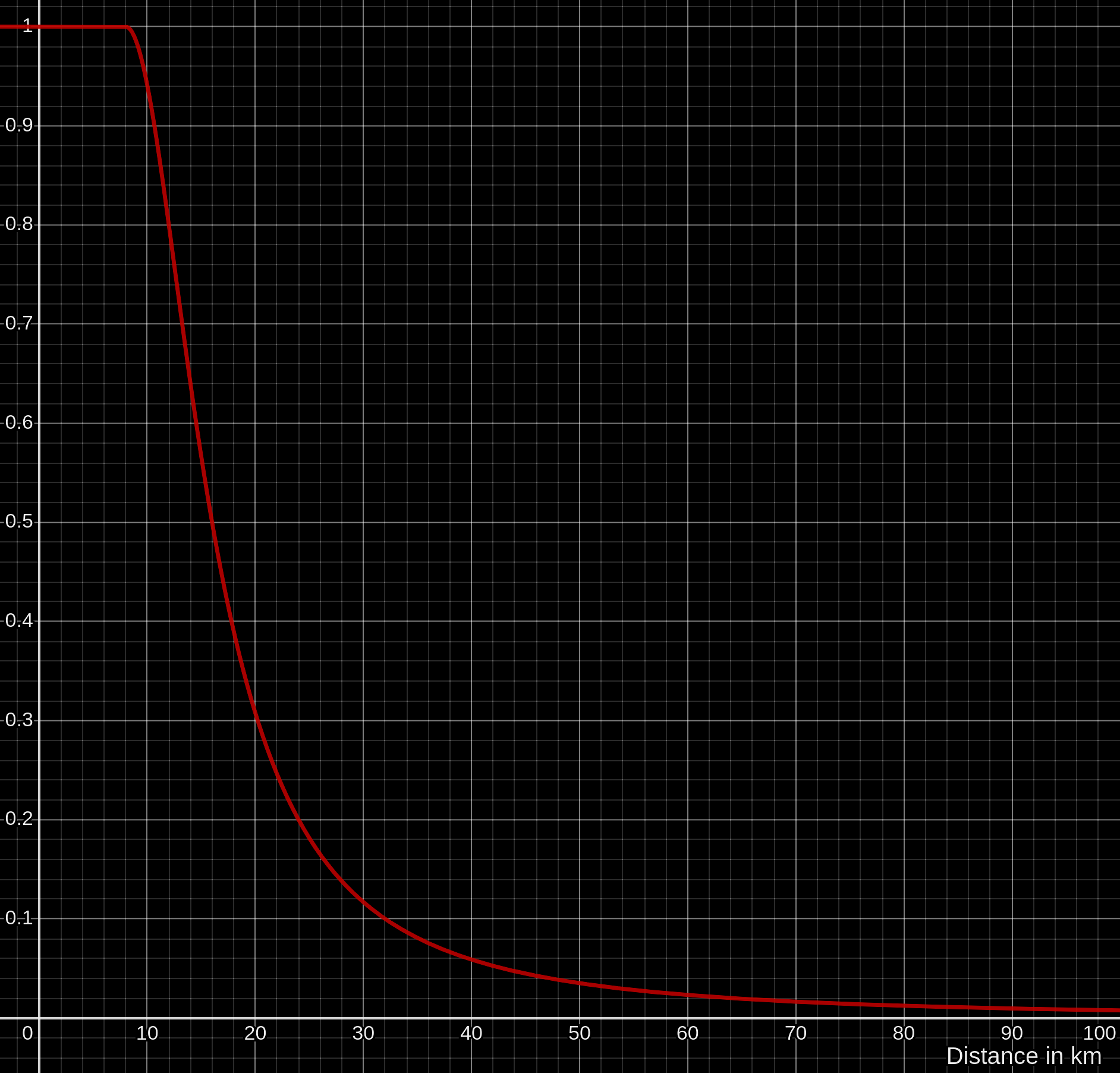
const auto collision_min_distance = 8'000.f; // meter

if(converging_velocity > 0.f) {
	const auto d = std::max(0.f, dist - collision_min_distance) / collision_min_distance;
	const auto alpha = std::clamp(1.f / (1.f + d * d), 0.f, 1.f);
	const auto force = direction * (alpha * converging_velocity / delta_time / 2.f);

	forces[origin] -= force;
	forces[dest]   += force;
}

Step 5: Simulate movement

Now that we know what forces are acting on each sub-plate, we just need to simulate their movement. The motion of each particle follows the well-known Newtonian equations of motion, which we will approximate numerically using Verlet integration because of a couple of key advantages:

• Similar computational complexity to implicit/explicit Euler integration, but with much better numeric stability
• Easy to implement, since we only need to keep track of the current and previous position
• Constraints are trivially easy to implement, by just modifying the calculated new positions. Which is important for us because we have to constrain each vertex to keep it on the sphere’s surface.

To update each vertex position $\vec{p}$ we use:

$$\vec{p}_t = \left \| \vec{p}_{t-1} + (\vec{v}_{t-1}\cdot \text{dt} + \frac{\vec{\text{force}}}{\text{mass}}\cdot \text{dt}^2)\cdot (1-\text{drag} \cdot dt) \right \| \cdot \text{radius}$$

Where $dt$ is the delta time between the two steps, $\vec{force}$ is the sum of all forces acting on the sub-plate, $mass$ and $drag$ are constants and $\vec{v}$ is the velocity, which is calculated after the positions are updated using:

$$\vec{v}_t = \frac{\vec{p}_t-\vec{p}_{t-1}}{dt}$$

Of course, because each sub-plate moves independent of the others, there will be some problems like self-intersections, which we’ll need to clean up afterwards. But that is a topic for another blog post.

Tectonic plates moving, colliding and being subducted.

Elevation

Now that we have continental and oceanic plates moving about, we can also use that information to finally pile up some mountains and create some actual terrain.

6. Update elevation

Mountain formation in reality is a complex process, involving 3D interactions and folding between parts of the crust with varying compositions and densities. But in our model this is simplified quite a bit and only depends on the sub-plates velocities and their Boundary_type.

In fact, there are only two types of boundaries that are relevant for mountain formation:

Boundary_type::collision

During collisions, the crust material between the two plates is pushed closer together. Since both plates are not dense enough to subduct they instead pile up, which forms large mountain ranges and plateaus, like the Alps or Mount Everest.

To simulate this process, each edge on a collision boundary is check and if the two plates are still converging, the crust around the boundary is lifted by an amount based on the converging velocity and its distance to the boundary. Since this affects not just the two vertices, that are part of the boundary, but also the crust that is further away, a flood-fill is used to recursively visit all neighboring vertices of the plate until the elevation change becomes insignificant.

My initial implementation actually contained a more general approach, that compared the volume of the Voronoi cell of every vertex, including internal ones, between time-steps and updated the elevation to preserve their volume, also taking the isostatic equilibrium into account. My hope was, that this would better simulate the effects of collisions further from the boundary. Alas, the resulting terrain was much more messy and noisy than the current implementation. But that is definitely an approach I plan to revisit once the simulation is stable and produces satisfactory results.

Boundary_type::subducting_*

The other type of boundary that contributes to mountain formation are subduction zones. In the partial melting process of the subducted crust, water and other foreign materials, that were pulled down with the bedrock, disrupt the equilibrium inside the upper mantle, which causes a sharp increase in volcanism on the un-subducted plate above. This process creates the long thin mountain ranges near subduction boundaries, like the Andes and the islands around the ring of fire.

The simulation for this is currently quite similar to that for collision boundaries, except that only one of the plates is lifted up, while the other one is pulled down, and that the position of the elevation increase is slightly different, i.e. a smaller area and slightly inland from the actual boundary.

9. Simulate Erosion

The elevation-code described above mostly adds elevation. So, if left to its own devices, the whole planet would be one huge mountain range. To balance this out, we need an additional system that reduces the elevation, which is precisely what the erosion simulation does.

This part is more or less copied as is from the paper of Cortial et al., with just some minor additions. Eventually, once we have a climate simulation to generate temperatures, precipitation and watersheds, we’ll extend this to a more interesting/faithful/complete erosion system. But for now, this simple simulation is good enough to counterbalance the mountain formation.

const auto ocean_elevation =  -6'000.f; // meter
const auto max_elevation   =  10'000.f; // meter
const auto min_elevation   = -10'000.f; // meter

const auto oceanic_dampening  = 6e-5f; // meter/year
const auto sediment_accretion = 3e-6f; // meter/year
const auto simple_erosion     = 8e-5f; // meter/year

const auto sink_amount   = 0.006f; // meter/year
const auto sink_begin    = 2'000'000.f; // years
const auto sink_duration = 2'000'000.f; // years

if(types[v] == Crust_type::continental) {
    // Move elevation of continental crust towards 0m above sea level.
    // Since this is based on the current elevation, larger mountains are eroded faster.
	elevation -= elevation / max_elevation * simple_erosion * dt;

} else if(elevation > -6'000.f) {
    // Oceanic ridges are initially less dense than the surrounding sea floor and
    //   cool and sink over time, which is (crudely) simulated here
	const auto age = now - created[v];
	if(age > sink_begin && age < sink_duration + sink_begin) {
		elevation = std::max(ocean_elevation, elevation - sink_amount * dt);
	}

    // Ocean floor above the height of the abyssal plane is pushed down
	const auto x      = elevation / ocean_elevation;
	const auto factor = (1.f - elevation / min_elevation) * smootherstep(0.f, 0.2f, x);
	const auto delta  = std::max(0.f, factor * oceanic_dampening * dt);
	elevation         = std::max(ocean_elevation, elevation - delta);

} else {
    // Ocean floor below the abyssal plane (e.g. from old inactive subduction zones)
    //   is slowly filled up by sediment.
	elevation += sediment_accretion * dt;
}

Conclusion

Now that we’ve got some movement going and elevation elevating, we’ve actually already covered half of the algorithm:

1. Add vertices where more details are needed and remove vertices unessential ones
2. ✔ Compare the properties of neighboring sub-plates to determine if they belong to the same tectonic plate or fall into one of the boundary zones discussed above (transform, divergent, convergent CC/OC/OO)
3. Create new oceanic crust at divergent boundaries
4. ✔ Calculate all forces acting on the sub-plates
5. ✔ Calculate the acceleration of all sub-plates, based on the forces acting on them, and utilize Verlet integration to calculate their new velocities and positions
6. ✔ Update each sub-plate’s elevation, if they are part of a subduction or collision zone
7. Check for collisions and resolve them
8. Check and restore Delaunay condition, if required ^[7]
9. ✔ Simulate erosion
10. Combine colliding continental plates and split plates that have gotten too large

All that’s left for the last two posts now, is to clean up the mess we left behind in step 5. Which means cleaning up inconsistencies in the mesh and handling collisions caused by the plate’s movement (7. and 8.) as well as creating/destroying crust (1. and 3.) and simulating large-scale plate interactions (10.).