Before we can get started with the actual generation/simulation algorithms we first need to decide how to store our data, i.e. how the world is represented in the data-model. Given that it’s not clear what algorithms, we will use later and what their requirements will be, we’ll want to choose an extendable model, that won’t restrict our options later.

There is however one decision we need to make right now, and that is what kind of shapes we want to support. As said in the previous post, I plan to focus on spherical worlds, seeing as the real world is (nearly) spherical^[1] and I want to be able to directly compare it with my results. Since we are — at least at the current scale — only interested in the information on the surface of our world, this means that we need an efficient way to store information for points on the surface of a sphere.

On a Sphere, triangles can have more than one right angle ^[source]

Working on the surface of a sphere brings with it a number of interesting problems^[2] because it’s not the kind of euclidean space we are used to from school, but an elliptic space. This doesn’t really affect us at human scale, but at the scale of continents we will need to take that into account when moving points on the surface and calculating distances and angles. Another problem with using a sphere for our world is that it limits our possible data structures because a sphere can’t be projected onto a flat surface without introducing distortions or other artifacts. So, simply projecting a bitmap texture onto the sphere is not really a practical course of action, if we want to avoid those problems.

But based on the other projects I’ve looked at and my requirements, a triangle mesh is the obvious choice, anyway. Structured Grids like bitmaps/2D-Arrays often suffer from artifacts, either from discretization problems or other limitations, that are less apparent on unstructured grids. A triangle mesh is also a promising data structure because it’s extremely flexible as far as the resolution is concerned, which will be required to support the relatively large detailed worlds I’m looking to generate.

So, the data structure of choice will be a triangle mesh of a Delauny triangulation (as well as its dual-graph, the voronoi diagram) with a variable resolution based on local detail requirements.

Mesh Data Structure: Quad-Edges

The next question is: How do we store this triangle mesh?

The simple option would be an array of faces, each containing the connected vertices. But to actually work with the mesh we’ll need an efficient way to traverse it, i.e. answer questions like “what other vertices/faces are connected to this vertex?”. Other common data structures for triangle meshes, that solve this problem, are directed edges, winged edges and half-edges.

But the data structure I’ve decided on are quad-edges, first described by Jorge Stolfi and Leonidas J. Guibas in 1985. Their main benefit is, that they model the primal triangle mesh, as well as its dual (voronoi diagram) at the same time. This means that we can traverse both and naturally switch between them if our algorithm requires it. Furthermore, quad-edges can answer many questions about the topology in constant time and often with just a simple bit-operation or by dereferencing a single pointer. And despite all, that their memory layout can be quite compact, which will be important for larger worlds.

The three main concepts are the same as for any mesh: vertices, faces and edges. Vertices are points on the surface and the element to which we will link most of our information like elevation. Two vertices can be connected by an edge, and three connected vertices form a single triangular face.

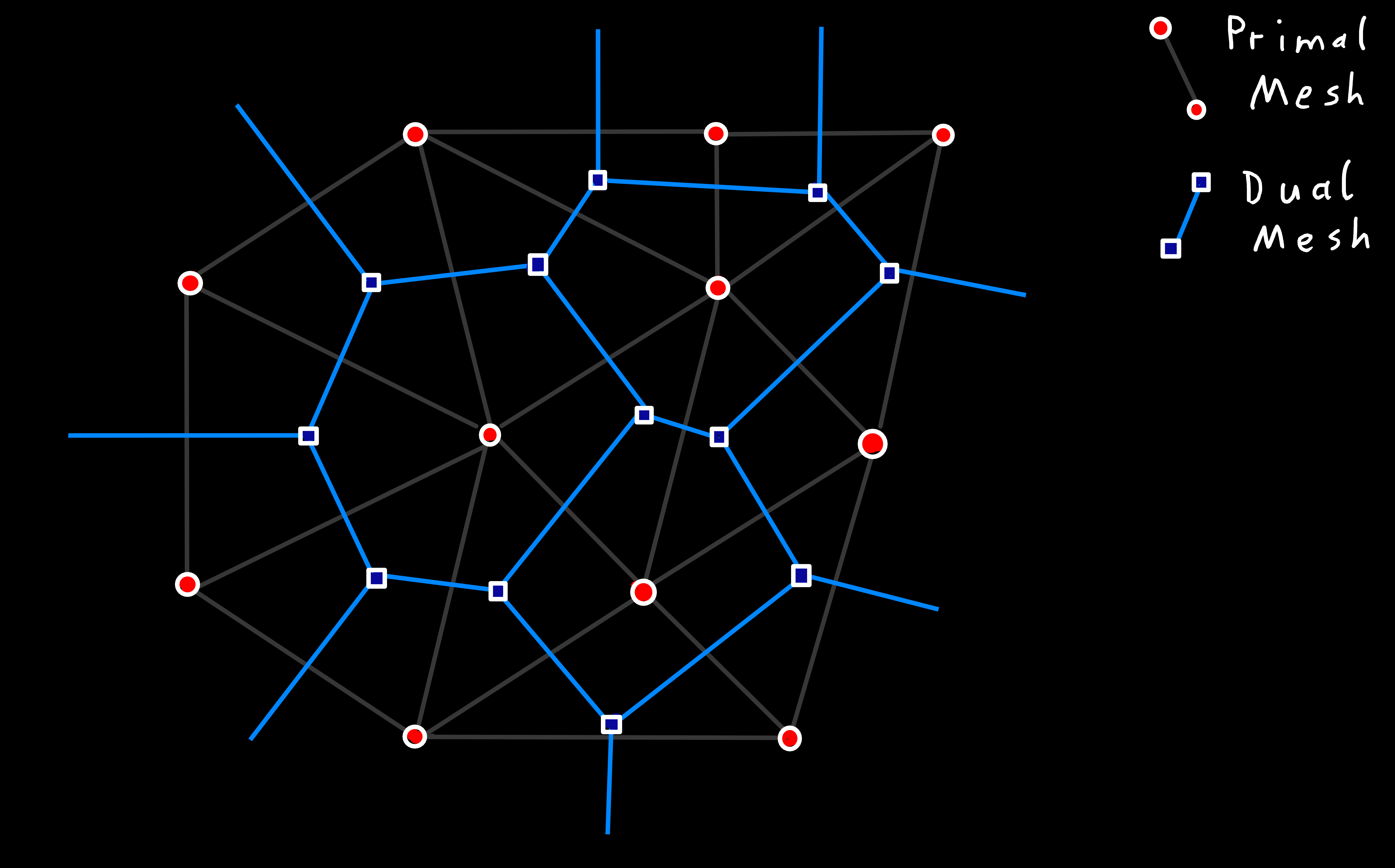
In addition to this primal mesh, we also want to work with its dual. Here vertices and faces switch places, that is each face in the primal mesh is a vertex in the dual mesh^[3], which are connected into voronoi cells with one of the primal vertices inside. As we can see in the image below, for each edge in the primal mesh (gray) the dual mesh contains an edge that connects the face on the left and on the right side of it. But the edges and vertices at the boundary are a bit of an edge case and form voronoi cells that are infinitely large. Luckily, that is a case we can ignore for now because our sphere is a closed mesh without any holes or boundaries.

The dual mesh is especially interesting for us because the voronoi cells define the area around each primal-vertex that is closer to it than any other vertex. Which is useful to calculate its sphere of influence or mass during plate simulation and will also prove useful for simulating drainage areas and rivers, later.

A Delaunay triangulation (grey) of the vertices (red) and its dual, consisting of the circumcenters of the faces (blue) and connecting edges (cyan), forming the voronoi cells.

Of these three concepts, the most important one for our quad-edge data structure is — as the name suggest — the edge. Our edges are directed, which means they know which vertex they are coming from, which one they are going to and which faces are on their left/right side. Thus, we need to store a total of four vertices for each pair of connected vertices, that form a quad-edge (see image below), to model the two possible directions of both the primal and dual mesh at that point.

Besides these pieces of information, we only need one other datum to describe the complete topology: Which edges start at a given vertex, i.e. the outgoing edges^[4]. And we store these as linked-lists of edges, where each edge knows the next edge around its origin, which is called an edge-ring.

This might look like a lot of information, but as we will see, most of it is redundant and doesn’t need to stored directly, but can instead be derived from the following and stored surprisingly compactly.

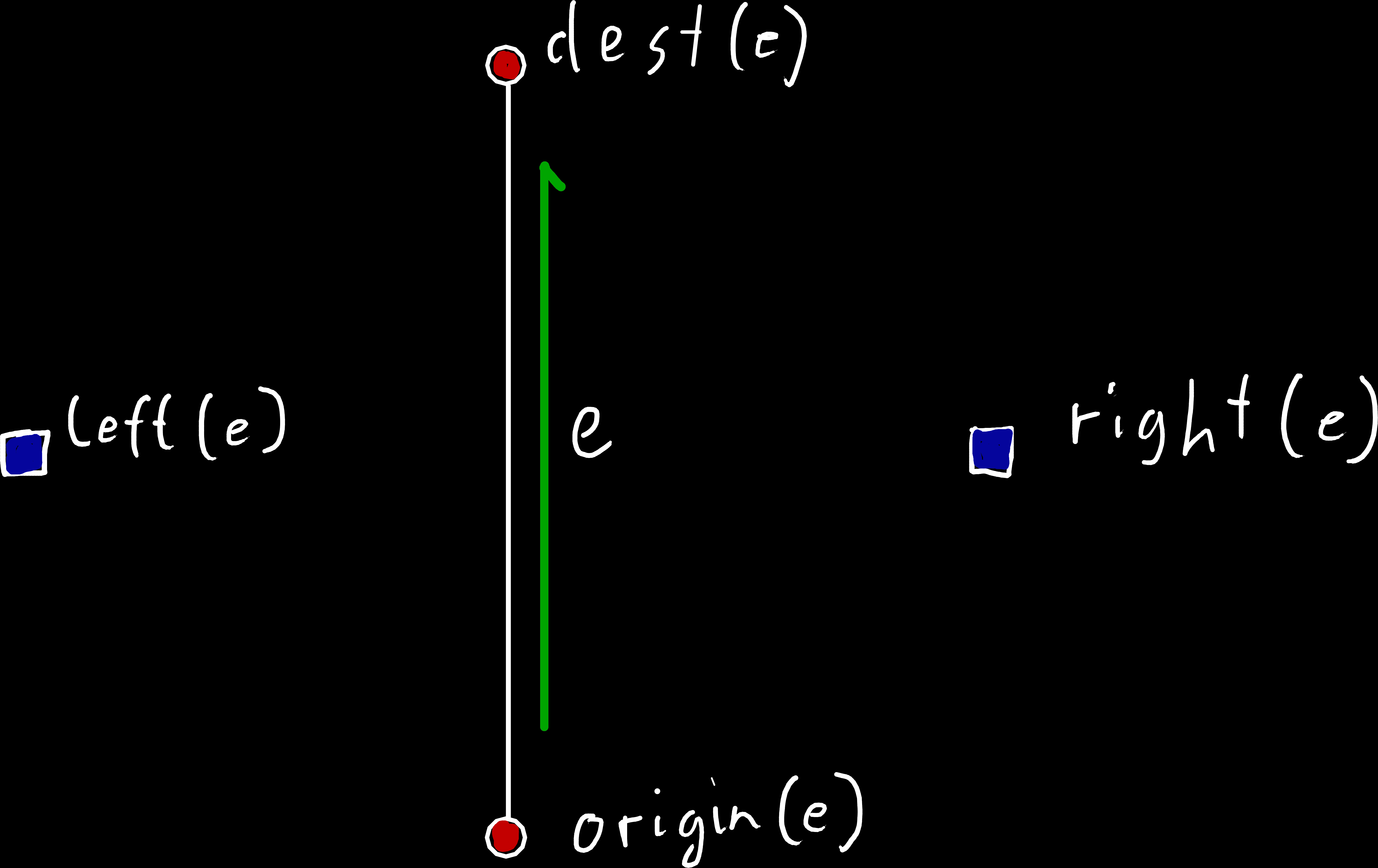
Each edge e knows its origin/destination vertex, as well as which face is on its left/right side.
Or origin/destination faces and left/right vertices for edges of the dual mesh.

Each edge also knows the other edges that are part of the same quad-edge, which we can access by rotating the edge counter clockwise.

Finally, each edge knows the next edge, when rotating counterclockwise around its vertex of origin, i.e. its edge-ring.

The information above describes the complete topology of our mesh, which we can access using the following basic operations:

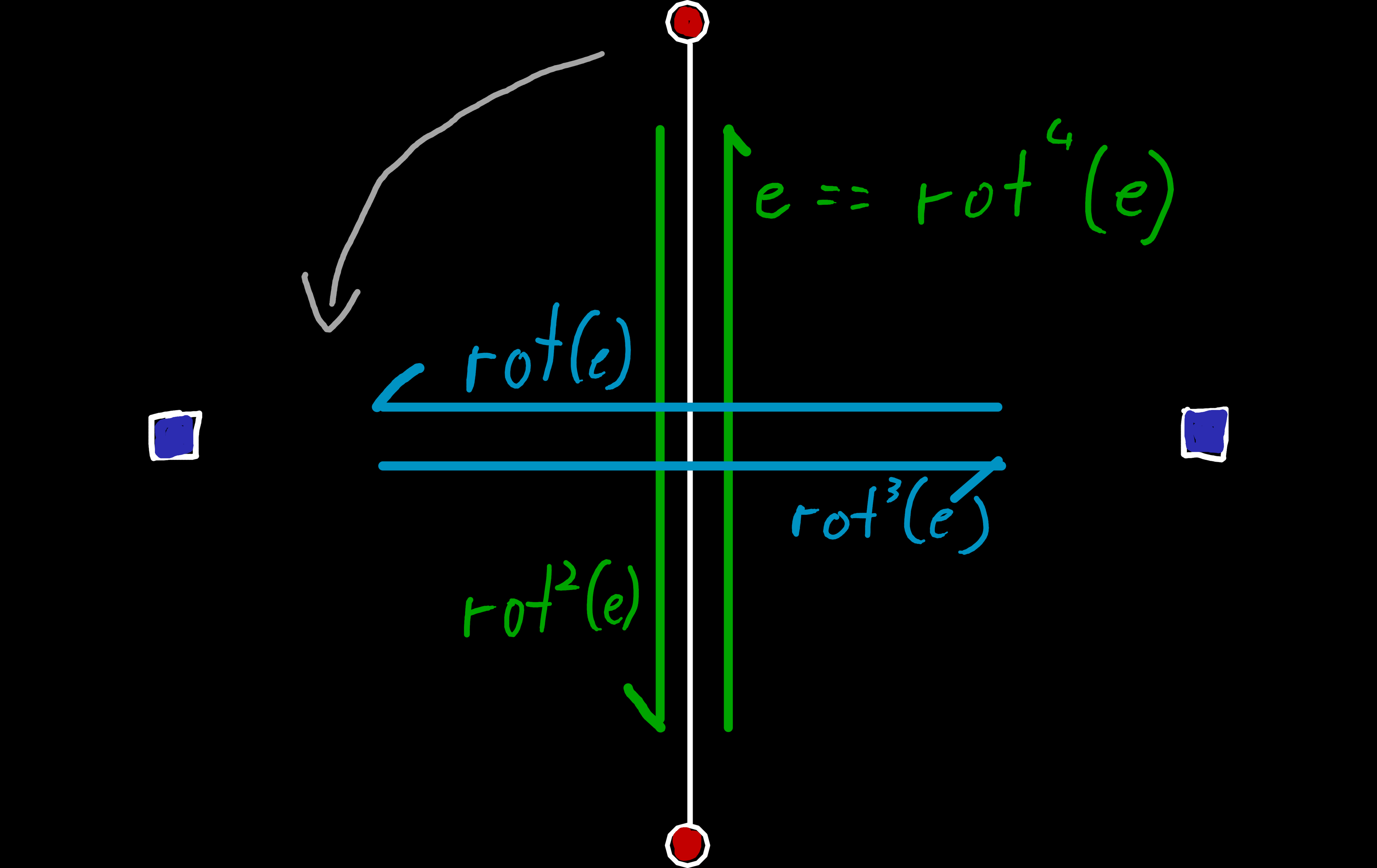
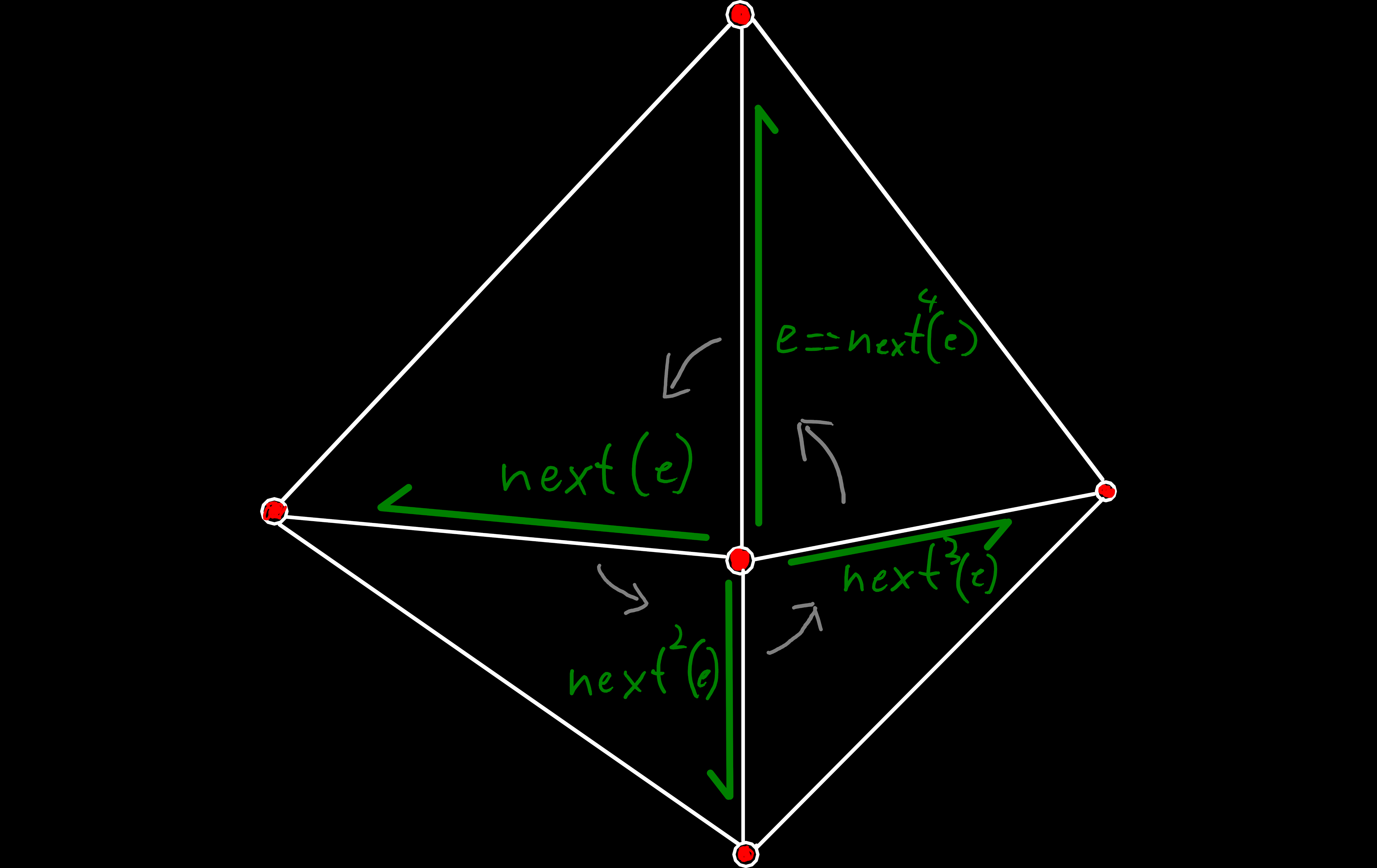
• origin(e): Gives us the origin of an edge (either a vertex in the primal or a face in the dual mesh).
• dest(e): Gives us the destination of an edge.
• left(e): Gives us the face/vertex on the left side of the edge.
• right(e): Gives us the face/vertex on the right side of the edge.
• rot(e): Gives us the next edge in a quad-edge. As each quad-edge consists of four edges, the result of the fourth rotation is our initial edge, again.
• sym(e): Gives us the edge that points in the opposite direction. So it’s the same as rotating the edge twice.
• origin_next(e): Gives us the next edge when rotating counterclockwise around the origin of an edge. Like rot(e) this will loop back on itself after we have visited every outgoing edge from the origin.

We can also combine these into more complex operations to traverse the mesh:

• dest_next(e): Same as origin_next(e) but gives us the next edge around the destination instead.
• left_next(e): Gives us the next edge rotating around the left face, i.e. left(e) will return the same value and the origin of the returned edge is our destination.
• right_next(e): Same as left_next(e) but rotates around the right face.

As we’ve seen, all operations above always rotate counterclockwise. So, the final operations we will define are variants of the above, that rotate in the opposite direction:

• inv_rot(e)
• origin_prev(e)
• left_prev(e)
• right_prev(e)

origin_next(e) allows us to iterate over all edges around a vertex or face. As with all operations the direction is counterclockwise and origin_prev(e) can be used for clockwise iteration.

Similarly, dest_next(e) can be used to iterate over all edges with a given destination.

And finally left_next(e) can be used to iterate over all edges that are part of a given face.

There is one more operation defined by the paper, that we will ignore here: flip(e), which returns the edge as seen from the other side of the polygon, i.e. the origin and destination stay the same but the left and right face are swapped. This operation is useful because quad-edges can actually represent any manifold polygon^[5], including non-triangular meshes and even non-orientable surfaces^[6], and don’t have an inherent preference for a specific side of the polygon. But we don’t really need that sort of flexibility for our endeavor, which is describing the topology of the surface of a sphere (and maybe later other simple shapes) and would rather trade it for some simplicity further down the road. So, what we will do instead is drop this operation and only work on one side of the polygon, defined by a consistent counterclockwise winding order.

Implementation

Now that we have seen how quad-edges describe the topology and what operations we need, we can start with the interesting part: Implementing it and looking for potential optimizations.

First, let’s reiterate what we need to store:

1. For each vertex: one outgoing edge (an edge where origin(e) is our vertex)
2. For each face: one edge going counterclockwise around the face (an edge where left(e) is our face)
3. For each edge:
   1. Its siblings, i.e. the three other edges that are part of the same quad-edge.
   2. The next edge, iterating counterclockwise around its origin (origin_next(e)).
   3. The origin/destination vertex and left/right face.

One thing we can drop immediately from that list is most of 3.3. Because each edge already knows the other edges of the quad-edge, we only really need to store the origin vertex/face of each edge. Everything else can be reconstructed from just these two, with:

• destination(e) == origin(sym(e))
• left(e) == origin(inv_rot(e))
• right(e) == origin(rot(e))

We could do something similar for the references to an edges siblings:

• sym(e) == rot(rot(e))
• inv_rot(e) == rot(rot(rot(e)))

But, as we will see next, that doesn’t really buy us anything because we can get rid of 3.1 entirely.

If we were to translate that naively to C++ it could look something like this:

struct Vertex {
	Edge* outgoing_edge;           // 1.
};
struct Face {
	Edge* ccw_edge;                // 2.
};
struct Edge {
	std::array<Edge*, 4> siblings; // 3.1.
	Edge*                next;     // 3.2.
};

// We need two separate types for edges, because the 
//   type of the origin is different for primal and dual edges
struct Primal_edge : Edge {
	Vertex* origin;                // 3.3.
};
struct Dual_edge : Edge {
	Face* origin;                  // 3.3.
};

struct Mesh {
	// The actual data, that is referenced by the pointers above
	std::vector<Vertex>      vertices;
	std::vector<Face>        faces;
	std::vector<Primal_edge> primal_edges;
	std::vector<Dual_edge>   dual_edges;
};

As this just defines the topology, we still need a way to store our actual data, like vertex positions or elevations. We could just add those to the struct as additional member variables, but that would mean that we need to modify them each time we implement a new generation algorithm, which would make future expansion more difficult^[7]. Hence, instead we will give each vertex/face/edge a unique ID, that we can then later use as a key to reference our data.

To define these IDs, we will just use their index position inside the std::vector that contains them. For vertices and faces this will work flawlessly, but for edges we also need to differentiate between primal and dual edges. To solve this problem, we will resort to the age-old tradition of stealing every bit that isn’t nailed down. To be precise, we will use the most significant bit of our ID to decide if it references a primal or dual edge^[8].

If we visualize that structure, we see another interesting effect. Because each edge always belongs to a quad-edge, if we add a new edge to our mesh, we will always need to create 4 edges (2 primal + 2 dual). So if we store and reference our edges as described above, we can find the siblings of an edge just by modifying their index, without storing any additional data.

                       quad edge 1               quad edge 2
                           ︷                        ︷
              ╭────────────┬────────────┬────────────┬────────────┬────────────╮
primal_edges: │     e0     │     e1     │     e2     │     e3     │     ...    │
              ╰────────────┴────────────┴────────────┴────────────┴────────────╯
              ╭────────────┬────────────┬────────────┬────────────┬────────────╮
dual_edges:   │     e0     │     e1     │     e2     │     e3     │     ...    │
              ╰────────────┴────────────┴────────────┴────────────┴────────────╯

Edge-index bits:
       ╭──┬──┬──┬──┬───┬──┬──┬──┬──╮
Bit:   │31│30│29│28│...│ 3│ 2│ 1│ 0│
       ╞══╪══╪══╪══╪═══╪══╪══╪══╪══╡
Value: │ 1│ 0│ 1│ 1│...│ 1│ 0│ 0│ 1│
       ╰──┴──┴──┴──┴───┴──┴──┴──┴──╯
         ↑                        ↑ 
         0 = primal edge          0 = 1. edge of quad-edge
         1 = dual edge            1 = 3. edge of quad-edge (== sym(e) == rot(rot(e)))

The 31st bit is reserved to decide if the edge belongs to the primal mesh or its dual, and the rest is used as the index into the respective vector. But because we allocate the edges continuously, they always come in pairs inside each vector, and we can switch between them by just flipping the 0th bit of their index. What this means is that we can not only drop the siblings member but that we can actually calculate rot(e), sym(e) and inv_rot(e) using relatively simple bit-wise math instead of chasing pointers!

Since we are already stealing parts of our indices, we will reserve one more value from each as an identifier^[9] for invalid or unset edges, vertices and faces. These will be important later to define boundary edges or incomplete meshes during construction. But they also allow as to “delete” elements from the mesh. Because the index of an element is also used to reference it, we can’t just remove them from the vector, as that would move all later elements, changing their index. Instead, we’ll utilize the invalid IDs to leave “holes” in the vector, that we can skip during processing and fill in later with new vertices/faces/edges.

And that’s it, for the most part. As a last step, we’ll just sprinkle a bit of data-oriented design over our structure, by moving our data from the Vertex/Face/Edge struct directly into separate vectors in the Mesh. That doesn’t change much in our case, as our structs were already rather small and simple, but could be a wee bit faster for some cases^[10]. And it also frees up Face, Vertex and Edge as type names, that we can then use as type-safe ID-wrappers^[11]. We also dropped the separate types for primal and dual edges, to further simplify the structure. However, it might be interesting to provide separate types to already distinguish them in the type-system, instead of later at runtime. But that is an extension I might look at later.

struct Face {
	uint32_t id;
};
struct Vertex {
	uint32_t id;
};
struct Edge {
	uint32_t mask;
};

class Mesh {
  private:
	friend struct Edge;
	
	std::vector<Edge>   vertex_edges_;
	std::vector<Edge>   face_edges_;
	
	std::vector<Vertex> primal_edge_origin_;
	std::vector<Edge>   primal_edge_next_;
	std::vector<Face>   dual_edge_origin_;
	std::vector<Edge>   dual_edge_next_;
};

Operations

We’ve already seen that we can implement rot(), sym() and inv_rot() as bit-wise operations on the ID, so that is the first thing we will implement^[12]:

inline constexpr auto edge_type_bit = uint32_t(1) << 31u;

struct Edge {
	uint32_t mask;
	
	// The default constructor sets all bits to 1,
	//   which is our representation for an invalid edge
	Edge() : mask{~uint32_t(0)} {}
	
	// And we also have constructors that take a mask 
	//   or construct a new one from an index and a bool 
	//   (i.e. set the highest bit if it's a dual edge)
	Edge(uint32_t mask) : mask{mask} {}
	Edge(bool dual, uint32_t index)
	  : mask{dual ? (index | edge_type_bit) : index} {
	}
	
	// If we need the actual index, we have to unset the highest bit
	uint32_t index()const   { return mask & ~edge_type_bit; }
	// And to decide if an edge belongs to the dual or primal mesh
	//   we can just shift it, so its highest bit is the only one left
	bool     is_dual()const { return mask >> 31u; }
	
	// A simple operation, we haven't talked about, which gives
	//   us the first edge of a quad-edge by unsetting both the highest and lowest bit.
	Edge base()const    { return { mask & ~(edge_type_bit | 1u)}; }

	// As we have seen above, the two primal/dual edges that
	//   belong to the same quad edge are always at an odd/even
	//   index and right beside each other.
	// So we just need to xor the least significant 
	//   bit to switch between them
	Edge sym()const     { return { mask ^ 1u}; }
	
	// rot and inv_rot are a bit more complex, because we need to change both bits.
	// First we always need to xor the highest bit, as rot always 
	//   alternates between dual and primal edges.
	// And we also need to change the lowest bit, which we will do
	//   with the second xor (see graphic below)
	Edge rot()const     { return {(mask ^ edge_type_bit) ^  is_dual()}; }
	Edge inv_rot()const { return {(mask ^ edge_type_bit) ^ (is_dual() ^ 1u)}; }

To implement the rotate operation, we need to change both the most and least significant bit. The most significant bit alternates between 0 and 1 as we alternate between primal and dual edges. But the least significant bit only changes every two steps. To implement this, its change is dependent on the most significant bit, i.e. we only alternate it if we rotate from a dual to a primal edge.

The next steps are the origin(e)/dest(e)/… operations to get the surrounding vertices and faces of an edge. The functions to get the origin vertex/face are relatively simple, as we just need to check if the operation is valid for this type of edge (primal vs. dual) and access the corresponding vector in the Mesh struct. And for the destination and the left/right face, we just have to rotate the edge appropriately beforehand and then get the origin of the result.

	Vertex origin(const Mesh& mesh)const {
		assert(!is_dual());
		return mesh.primal_edge_origin_[mask];
	}
	Vertex dest(const Mesh& mesh)const {
		return sym().origin(mesh);
	}
	
	Face origin_face(const Mesh& mesh)const {
		assert(is_dual());
		return mesh.dual_edge_origin_[index()];
	}
	Face dest_face(const Mesh& mesh)const {
		return sym().origin_face(mesh);
	}
	
	Face left(const Mesh& mesh)const {
		return inv_rot().origin_face(mesh);
	}
	Face right(const Mesh& mesh)const {
		return rot().origin_face(mesh);
	}

Next are the functions to actually traverse the mesh. origin_next(e) is again quite simple — determine the correct vector based on the type of the edge and load the corresponding next pointer — but implementing all the others in-terms-of it is a bit more complex and perhaps needs a bit of visualization:

	Edge origin_next(const Mesh& mesh)const {
		return is_dual() ? mesh.dual_edge_next_[index()]
		                 : mesh.primal_edge_next_[index()];
	}
	Edge origin_prev(const Mesh& mesh)const {
		return rot().origin_next(mesh).rot();
	}
	Edge dest_next(const Mesh& mesh)const {
		return sym().origin_next(mesh).sym();
	}
	Edge dest_prev(const Mesh& mesh)const {
		return inv_rot().origin_next(mesh).inv_rot();
	}
	Edge left_next(const Mesh& mesh)const {
		return inv_rot().origin_next(mesh).rot();
	}
	Edge left_prev(const Mesh& mesh)const {
		return origin_next(mesh).sym();
	}
	Edge right_next(const Mesh& mesh)const {
		return rot().origin_next(mesh).inv_rot();
	}
	Edge right_prev(const Mesh& mesh)const {
		return sym().origin_next(mesh);
	}
};

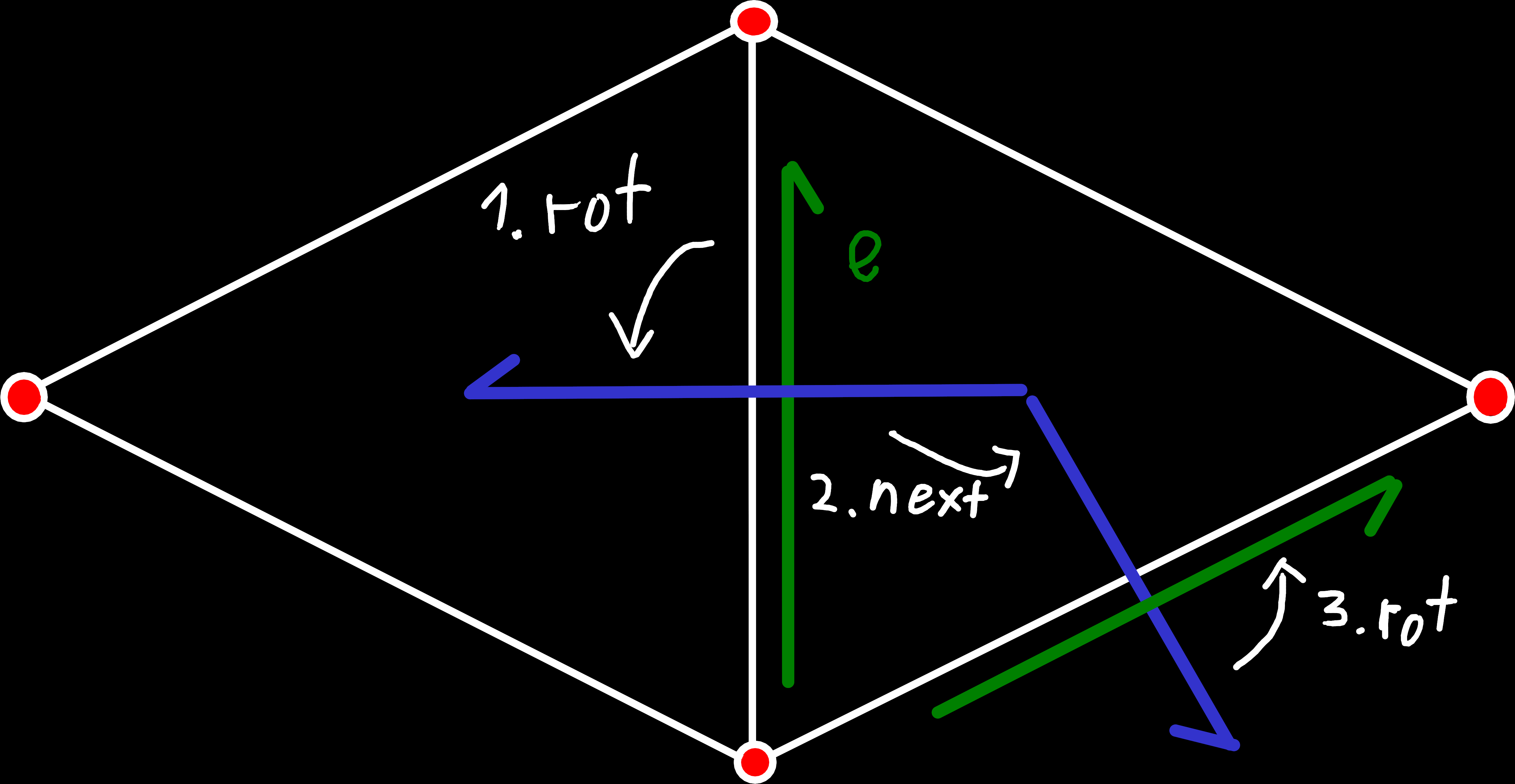
One example for the methods above, that shows how origin_prev() can be implemented in terms of origin_next().

The key here is that we first rotate the edge, to get the dual edge that points from the right to the left face. Just like with primal edges, we can use origin_next() to get the next (counterclockwise) edge around the origin, but for dual edges that origin is a face instead of a vertex. So, when we rotate our dual edge, we get the dual edge that point “through” the next edge of the right face or in other words origin_prev() of our original mesh. And to get the primal edge, we are actually looking for, we then just need to rotate the dual edge again.

Higher Level Abstractions

Based on these relatively simple operations, we have seen so far, we can now construct higher level abstractions to navigate the topology. One operation we need relatively often is iterating over every neighbor of a given vertex^[13], which can be implemented as:

// Get any edge that points away from the vertex
auto edge = vertex.edge(mesh);
auto e    = edge;
do {
	// Get the destination vertex of the current edge
	auto v = e.dest(mesh);
	
	// Do something with v
	
	// Get the next (CCW) edge
	e = e.origin_next(mesh);
	
	// If the next edge is the one we started with,
	//   we have visited all edges and can stop
} while(e!=edge);

Precisely because this is a common operation, the actual API provides iterators and methods that simplify the above code to:

for(auto v : vertex.neighbors(mesh)) {
	// Do something with v
}

One part of the API we’ve ignored so far is how we construct a mesh to begin with. And for some algorithms, we will also need to be able to modify an existing mesh. The operations we will need for this are:

• Create a new triangle face that connects three vertices
• Flip the central edge of two adjacent faces, i.e. remove the shared edge and replace it with a new edge between the two previously unconnected vertices
• Split an edge into two edges, inserting a new vertex and new faces between them
• Collapse an edge, i.e. merge two vertices and remove the edges and faces between them

But because these operations are a bit more complicated and this post is already far longer than I originally planned, we will look at that in a future post.

Positions, Elevations and other Additional Information

However, there is one part we still have to talk about. Everything we have looked at so far is purely concerned with the topology — which vertices/faces are connected to each other — and isn’t concerned about how it’s actually laid out in space. That is, if it can be laid out without intersecting itself, it doesn’t matter if our basic shape is a sphere, cube, plane or tesseract^[14].

But even if our data structure isn’t concerned about the positions in space, we still do care about that for many applications and need a way to store them. We’ve already touched on the fact that we can use the IDs of our vertices/faces/edges to link them to additional information like elevation or temperature, and we will handle their positions in exactly the same way. Because our elements are laid out in a continuous vector in memory^[15] and our IDs are based on their position, we can also just use a vector for our addition data and use the IDs to index into them.

While that will work, there is a bit more complexity, to handle changes when we modify the mesh later. And a bit of validation and type-safety would also be a welcome addition. To achieve that, we will create a new Layer type that stores information linked to a given part of our mesh, that looks like this^[16]:

enum class Layer_type {
	vertex, face, edge_primal, edge_primal_directed, edge_dual, edge_dual_directed
};
	
template <typename T, Layer_type Element>
class Layer {
  public:
	// Access the data for a specific element
	// The parameter type is Vertex, Face or Edge depending on the Layer_type
	T&       operator[](type<Element>);
	const T& operator[](type<Element>)const;
	
	size_t size() const;
	bool   empty() const;
	
	// begin() and end() so the type can be used in range-for loops
	T*       begin();
	const T* begin()const;
	T*       end();
	const T* end()const;

  private:
	// ...
};

Because Layer is a class template, it can be used to store all kinds of different data types^[17] and can reference vertices, faces and all types of edges.

One thing that might be a bit surprising at first is the number of possible types of edges in Layer_type. In addition to the distinction between primal and dual edges, we also differentiate between directed and undirected edges here. While the edges in our mesh are always directed, much of the information we might want to store about them will be identical for both directions. For example, when we model plate tectonics and store the distance between neighboring vertices, we would choose edge_primal instead of edge_primal_directed and only require half the memory to store our data.

Not all data is directly related to parts of the mesh or might be so sparse that a continuous storage doesn’t make sense. For these cases, there will also be unstructured data layers, that model a simple key-value store, which I might talk about later.

World Class

As already noted, the Layers might need to be updated whenever the mesh is modified, which means both are heavily intertwined. Thus, it isn’t really feasible to construct them independently of each other. Hence, we will encapsulate both in a World type that manages both the Mesh and any created Layer:

class World {
  public:
	const Mesh& mesh() const;
	Mesh_lock   lock_mesh();

	const Dict*             layer(std::string_view id) const;
	Unstructured_layer_lock lock_layer(std::string_view id);

	template <typename LayerInfo>
	const typename LayerInfo::layer_t* layer(const LayerInfo& info) const;
	
	template <typename LayerInfo>
	Layer_lock<LayerInfo> lock_layer(const LayerInfo& info);

  private:
	// ...
};

In contrast to the types we have seen previously, the const and non-const getters are rather different here and also have different names. Because a complete World will be a pretty large and complex object with many layers, it is not feasible to copy it often. But creating copies of the current state of a World will be required later to implement an undo/redo functionality in the editor. To solve this, the World class implements copy-on-write semantics for the objects it contains. That means when a World is copied it still references the data of the original and only when one of them is modified the affected data — and only it — is actually copied. But to track these modifications, we need a bit of machinery, provided here by the ..._lock classes and lock_... methods. This recording of modifications will also allow us to check when the underlying data has been modified and for example cache the textures and vertex buffers used by the renderer.

Besides the mesh() getter, the class also contains two getters for layers, one for simple unstructured layers — that just have a name — and one for our more complex mesh-based layers.^[18] The latter is again a template, which hopefully is not that surprising because our Layer was also a template. But the parameter of the method probably warrants some further explanation. Every layer has a name with which it’s referenced in the procedural generation code, but it also has additional metadata linked to it:

1. The type of the data that it stores (T template parameter in Layer)
2. What its data is linked to in the mesh (Layer_type)
3. The initial value of its data (used both when it’s first created and when a new vertex is added to the mesh)
4. The range of valid values (only positive numbers, only numbers between 0 and 10, …)
5. Whether its data should be automatically validated against this range, to detect runtime errors
6. How the data should react to changes of the mesh (e.g. when an edge is split, should the value for the new vertex be interpolated between the original origin and destination, reset to the initial value, use the min/max of the values, …?)

Layers will usually be shared between multiple independent modules, that contain the actual procedural generation code. In fact, they are the main way of communication between them. Because it would be impractical to keep all of them synchronized, the system remembers all information about a layer at the time of creation. So, all later modules that want to access an existing layer only need to pass the first two points from the list above (which are validated against the stored information) and all others will be ignored.

Therefore, we also introduce a new type Layer_info to describe what a layer looks like and how it should behave, which can be constructed and then used to retrieve a concrete layer from the World:

constexpr auto position_layer = Layer_info<Vec3, Layer_type::vertex>("position");
constexpr auto distance_layer = Layer_info<float, Layer_type::edge_primal>("plate_distance")
                                .initial(-1.f);

auto [positions] = world.lock_layer(position_layer);

// Once we have the layer, we can access its data with the operator[] defined in the Layer class 
positions[Vertex(42)] = Vec3{10.f, -2.f, 3.f};

Conclusion

That is all for now, as I think this post is already a bit too long and complicated. We now just have to look at how meshes can be created and modified, before we can start with the really interesting parts.