Well, that was a bit of a longer pause, than I had hoped. So much for my “best intentions of documenting my progress”…

But I’ve finally managed to implement a working prove-of-concept for the plate simulation to generate terrain, also it’s still a bit rough around the edges.

Plate simulation (5x speed-up), consisting of about 2'500 triangles

While there are still many problems that need more work^[1], the general approach appears to work, at least.

But one thing that I noticed now is that the current tooling to visualize the results is not enough to test and debug the algorithm. So, before I continue working on the algorithm itself, I’ve decided to refactor and improve the editor to better visualize the generated data and allow users to modify the intermediary results. But first, it’s probably a good idea to document how the current implementation of the plate simulation works^[2].

The plate simulation in its current form is heavily inspired by the work of Cortial et al. in their 2019 paper Procedural Tectonic Planets. However, there are some aspects where my implementation diverges. Either because the paper didn’t provide details about a specific part of their implementation or because I think it will fare better, with my specific goals in mind.

Procedural Tectonic Planets

As the algorithm is relatively complex, I’ve split this post into multiple entries. In this one, we’ll look at how the tectonic plates are modelled and get an overview of the simulation on an abstract level and the following posts will then go into more detail about

• The generation of the initial state (i.e., the planet and its plates, that we use as input for the actual simulation)
• How plates are moved across the sphere’s surface and how that effects the elevation
• How collisions and intersection between plates are resolved and when/how new crust is generated
• When and how plates are merged or split (i.e. suturing and rifting)

Enough plate tectonics to be dangerous interesting

But first, let’s recap what I want to achieve with the plate simulation. The main focus of this step is to generate high-level terrain features, that look as realistic as possible^[3], at a resolution of about 1000 km² per data-point. Of course, for any practical use-case, as well as features like rivers, we’ll need a much higher resolution. My hope is that (similar to Undiscovered Worlds and the followup paper by Cortial et al. from 2020 “Procedural-Tectonic-Planets”) I will be able to later generate a more detailed small-scale view, based on the output of this high-level simulation.

To achieve these realistic results, I planned to stray as little as possible into the fun and easy, but unpredictable and boring world of random noise. Instead, I wanted to try to stay as close as reasonably possible to the physical reality^[4]. The problem with that is that plate tectonics is actually a quite complex 3D problem^[5] and a bit difficult to observe at the time-scales I’m interested in. So, I obviously can’t really hope to accurately simulate even a couple of years of plate movement on my target hardware, much less the millions of years I’ll need.

Luckily, I only really want to fool humans. So, the algorithm doesn’t have to be perfect, but only slightly more capable than the average observer and (as others have already demonstrated) I should be able to ignore a surprising amount of the more complicated aspects and only focus on some of the more obvious high-level features.

Plate-Interactions and the Wilson Cycle

The one thing I definitely can’t avoid to model are the tectonic plates themselves. So first, I should probably summarize what I understand about the physical processes, before I explain how I simplified them for my model^[6].

Tectonic activity map of the Earth^[source]

Tectonic plates are disjointed pieces of the Earth’s crust, that “float” on top of the mantel. Their movement is driven by convection currents in the upper mantle, that are in-turn influenced by the properties and interactions of the plates above. A common misconception^[7] is imagining the plates as solid ridged stone slabs, that float on top of liquid magma. Also, this a nice simple visualization, it’s important for their interactions to understand that both the crust and the mantel are actually solids. It is only over these long geological time-scales that the mantle behaves similar to a high-viscosity fluid. But over these time-scales, the crust also exhibits less rigid and more elastic properties, which enables some of the deformations we observe.

A nice simple model, that nonetheless contains all the high-level aspects I’m interested in, is the Wilson Cycle, that describes the formation and breakup of supercontinents as a series of stages.

Visualization of the Wilson Cycle^[source]

One essential factor in this model is the density of the crust that makes up the tectonic plate. While their composition is again quite complex, the crust can be classified into two general types: Continental crust, that has a relatively high density and makes up most of the dry landmass, and oceanic crust, that has a comparatively high density and makes up most of the deep ocean floor. Because the crust floats on top of the mantle, its density not only determines “how high” it floats, but also how it behaves when it gets thicker or thinner and how it reacts to collisions with other plates.

It’s important to note here, that this distinction is not as cut and dry as one might hope. Instead, it’s more of a categorization, based on the density of the average composition of the crust in an area. Which means, while there are some plates that consist mostly of continental/oceanic crust, most plates consist of both (as can be seen on the map above). And It’s also not uncommon for oceanic crust to end up on dry land, as well as for continental crust to be part of an ocean. But to keep the following descriptions as concise as possible, I’ll use the terms “continental plate” to describe a plate that mostly consists of low-density material in the relevant area and “oceanic crust” for high-density.

Considering all this, there are five types of interactions between plates we need to model:

Transform boundary: Two plates moving past each other^[source]

Divergent boundary: Two plates moving away from each other^[source]

Convergent boundary (CO): An oceanic and a continental plate colliding with each other^[source]

Convergent boundary (OO): Two oceanic plates colliding with each other^[source]

Convergent boundary (CC): Two continental plates colliding with each other ^[source]

Transform boundaries mostly just cause earthquakes, and are therefore not really of interest to us. So, we only have to look at convergent and divergent boundaries.

Divergent boundaries are relatively simple. The two plates move apart and mantel material wells up between them, which begins to a new ocean, once they have moved sufficiently far apart.

The most interesting boundaries are the convergent once, which we have to further distinguish into three subtypes based on the density/type of the involved crust:

• Continental-Oceanic (CO): The type of boundary we can see in the animation above. Here the denser oceanic plate is subducted under the continental plate, forming a trench between them, and starts to sink into the mantel. Once the subduction started, the weight of the already subducted plate also pulls on the remaining part, further speeding up the process. As the water subducted with the plate lowers the melting-point of the mantle material, it begins to partially melt, causing magma to rise and a volcanic mountain range to form^[8].
• Oceanic-Oceanic (OO): Quite similar to CO boundaries, except that the two plates are much more similar in density. But the principle remains the same, meaning the higher-density plate subducts, which will usually be the older of the two. This type of collision forms deep oceanic trenches and island arcs.
• Continental-Continental (CC): In contrast to the other two, there is no significant subduction here because both plates are too low-density to sink into the mantel, and are instead uplifted to create large mountains like the Himalayas.

Another interesting aspect, that is currently not implemented, is the formation of mid-plate volcanos, like the one that formed the Hawaiian islands. These are not caused by plate interactions, but are instead thought to be fed by hotspots in the mantle. Hence, they are mostly stationary and cause island arcs to form, when the crust above them moves.

Discretization of Space

The most obvious simplification in my model is that I’m using an extremely coarse discretization of the simulated space. In this step, I only really care about the rough shape of tectonic plates and large mountains, which doesn’t require much in terms of resolution.

As I’ve already outlined in the previous blog posts, I’m modelling my planets as triangle meshes with data stored on the vertices, faces and edges, instead of a more structured/uniform grid. This allows for a dynamic adjustment of the resolution in interesting (i.e. especially active) areas, without having to store detailed data about large stretches of empty boring ocean.

The simulation at the top consist of about 2’500 triangles and 1’300 Vertices, that are more or less evenly distributed on the surface (510’064’471 km²), which gives us a resolution of about 400’000 km² per Vertex.

One of the next steps will be to improve the subdivision algorithm, so I’ll end up with about 1’000’000 km² in mostly empty/flat areas and 1’000 km² - 100’000 km² near the coastline and mountains.

Reduced Dimensionality

There is one more way we can reduce the space we need to simulate: reduce the number of dimensions

While actual plate tectonics is a complex 3D problem — with complicated fluid dynamics and the isostatic equilibrium determining how plates interact and how high/low pieces of crust “float” — in this simplified model we can ignore most of this and only focus on the position of the plates on the surface and their elevation.

Visualization of the tectonic plates, consisting of multiple sub-plates, each with their own velocity, type, and elevation

To summarize, the planet is modelled as a triangle mesh^[9] where each vertex describes the properties of the crust in the surrounding area. To form tectonic plates, multiple connected vertices are grouped together by assigning them an integer ID. Or put another way, the vertices describe sub-plates, that are part of a larger tectonic plate.

So, each vertex stores the following information:

• The ID of the plate it belongs to
• Its elevation, i.e. the average elevation of this area’s crust (negative for areas below sea level)
• If it contains (mostly) continental or oceanic crust
• Its velocity
• When the crust formed, i.e. how old it is

Since each vertex is connected by an edge to its nearest neighbors, forming a Delaunay triangulation, we can inspect this mesh to detect collisions, traverse the plates and store additional information required for the simulation on its edges.

This is also one of the major differences to the work of Cortial et al., since they appear to store each plate as an individual spherical triangulation of points, instead of one coherent mesh. While keeping the plates as separate triangulations would simplify some parts of the algorithm (collision detection/resolution) my hope is that a single coherent mesh will make it easier to reuse the structure for both other simulations (water-shed, weather patterns, …) and rendering.

Simulation

On the simplest level, all we are doing to simulate plate tectonics is moving vertices around on the sphere’s surface and handle collisions by adding/removing vertices, changing the topology or modifying their elevation.

The movement itself is extremely simple. Since the vertices already know their position and velocity, all we need to do is apply the well-known equations of motion to calculate their new position on each time-step with: $x_{n+1} = x_n + v_n t + a_n t^2$

Some vertices belonging to different plates (green/blue), as well as their velocities, connections and a visualization of some of the forces that affect them: Orange spring-damper systems between vertices of the same plate and red force-generators between different plates, that pull/push vertices based on more complicated rules.

The interesting part is how we determine the vertices (i.e. sub-plates) accelerations $a_n$. This is the second part where we deviate from the work of Cortial et al., in part because of our different data model. Since all vertices are part of the same Delaunay triangulation, we can make the simplifying assumption that a vertex is only significantly affected by its direct neighbors, without introducing too many noticeable errors. Hence, we can use the same general system to calculate both the interaction between sub-plates belonging to the same tectonic plate and interactions between different plates.

This system can be thought of as similar to a spring-damping model based soft-body simulation. The vertices are treated as point masses, and each edge applies a force on its origin and destination based on its properties and the type of boundary the edge represents:

• Both vertices belong to the same plate: The force is calculated by a damped spring, that causes the sub-plates to retain their initial distance but allows for some deformations.
• Divergent boundary: A small ridge-push force is applied, that moves the vertices further apart.
• Convergent boundary (CC): A force, proportional to the velocity along the convergence direction and the distance between the plates, is applied to resist the collision until the plates either separate again or are sutured together.
• Convergent boundary (OC or OO): The denser of the two sub-plates is slowly subducted under the other and a force is applied to the subducting plate to simulate the slab pull

Forces are not just modelled based on the primal edges (gray lines), but also for their duals (dashed white line), which connect the faces and the left/right of the primal edge. But in this case, they are modelled as springs which connect the left and right vertices.

It should be noted that that model outlined here would not work for soft-body simulations, in the general case. Because we rely exclusively on the triangle edges to calculate forces, we are missing many springs that should normally be present in such a system, to prevent shearing and bending. However, in our case we avoid such artifacts because the individual vertices are (a) constrained to the sphere’s surface, (b) cover the whole sphere and we (c) prevent self-intersections and non-manifold geometry. This effectively limits the simulation to 2D, also the surface itself is a 3D sphere, and doesn’t allow for bending, folding or significant shearing, which would otherwise occur.

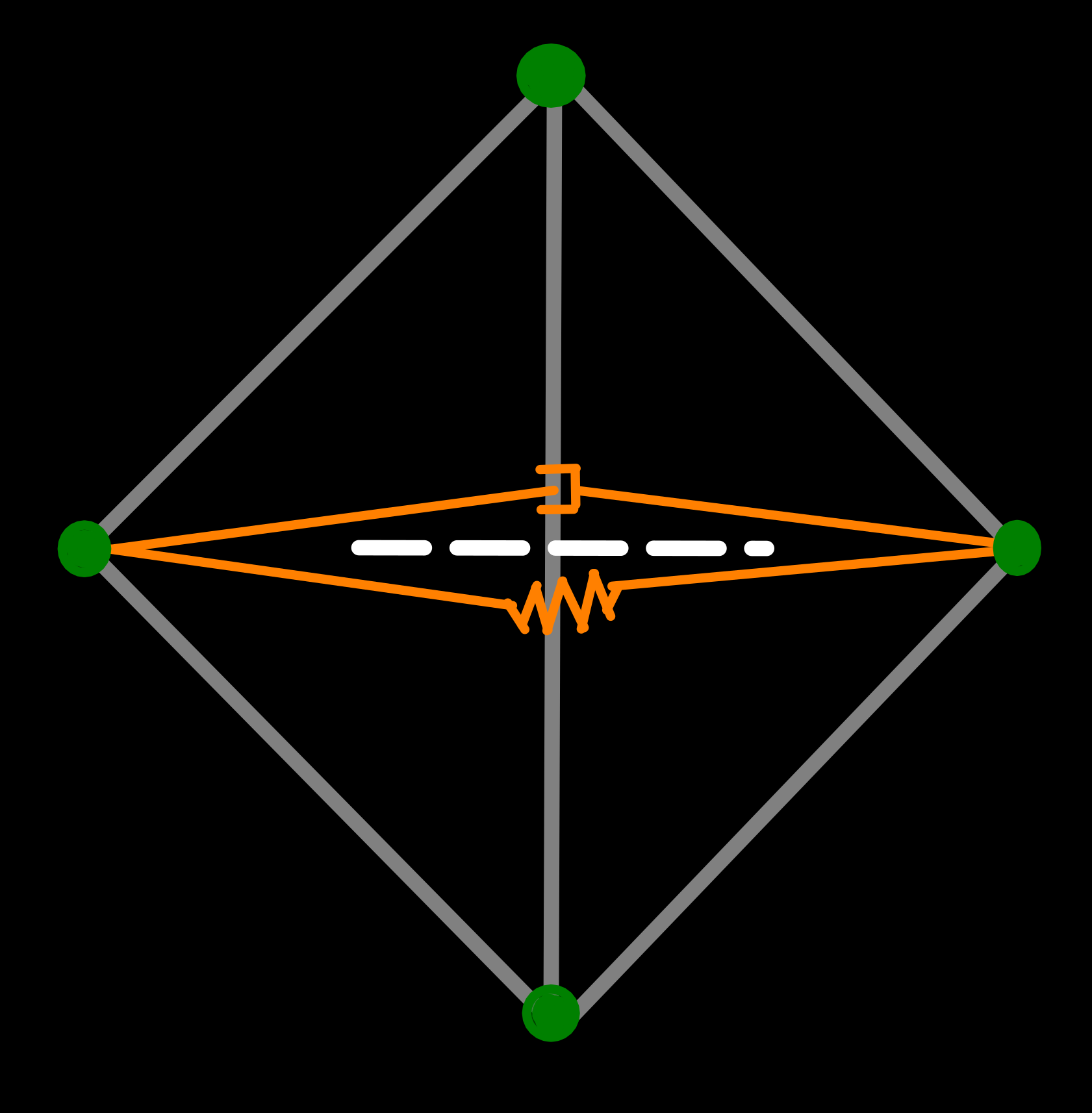
However, using just the edges of the primal mesh is not sufficient because of another reason: During the simulation the mesh is continuously updated, which includes flipping edges. Since this effectively removes springs, which are potentially under compression/tension, from the model and adds new ones, between formally unconnected vertices, which would then be in a relaxed state, this would create artifacts like heavy deformation of continents or loss of land area^[10]. To solve this, we don’t use only primal but also dual edges, which apply forces to the two vertices opposite of the corresponding primal edge (see image above). Because of this, when an edge is flipped, the spring-parameters can be swapped between the primal and dual edge, thereby conserving the spring’s stored energy and avoiding these kinds of artifacts.

Apart from the plate movement itself, there are also some other steps we need to take care of, that will be the focus of the next posts:

• The elevation of each sub-plate is updated near convergent and divergent plate boundaries, based on their separating velocities.^[11]
• Moving the vertices sometimes causes self-intersections of the mesh, that have to be fixed by removing one of the vertices. Since all triangles are restricted to the sphere’s surface and have the same winding-order, these artifacts can be detected by checking if a face has been inverted, i.e. its normal points in the opposite direction than the sphere’s surface normal.
• The vertices’ movement also frequently causes the Delaunay condition to be violated, which means we have to check and possibly restore it after each iteration. Since the number of violations is usually small, this is currently done by flipping edges that don’t pass the circumference-condition until the Delaunay triangulation is restored.
• And finally, there are steps that create/destroy vertices, either because of rifting/subduction or because an area needs more/less detail and thus vertices per km².

[Algorithm-Outline] After this high-level overview, here are the detailed steps each iteration of the simulation goes through, which the next couple of posts will look at in more detail:

1. Add vertices where more details are needed and remove vertices unessential ones
2. Compare the properties of neighboring sub-plates to determine if they belong to the same tectonic plate or fall into one of the boundary zones discussed above (transform, divergent, convergent CC/OC/OO)
3. Create new oceanic crust at divergent boundaries
4. Calculate all forces acting on the sub-plates
5. Calculate the acceleration of all sub-plates, based on the forces acting on them, and utilize Verlet integration to calculate their new velocities and positions
6. Update each sub-plate’s elevation, if they are part of a subduction or collision zone
7. Check for collisions and resolve them
8. Check and restore Delaunay condition, if required ^[12]
9. Simulate erosion
10. Combine colliding continental plates and split plates that have gotten too large

Conclusion

To summarize, the algorithm is heavily based on the 2019 paper Procedural Tectonic Planets by Cortial et al., with the following noteworthy modifications:

• The plates are not modelled as individual triangulation, but instead the complete planet forms a coherent triangle mesh, whose topology is continuously updated during the simulation. My hope here is that this will be more suitable for later simulations and allow for an easier integration with other parts of the system, even though it sadly makes the actual plate simulation a bit more difficult.
• Since the paper’s focus is the interactions between plates, the implementation of the movement itself was sadly not describes in any detail. Because of this — and enabled by the different triangulation approach — I’ve chosen to model the plate’s movement similar to a particle-based soft-body simulation. This should also allow for more plastic behavior and interesting deformations of plates during collisions.
• The last difference, that I’ll discuss in one of the following posts, is that collisions between plates are handled differently. Instead of resolving collisions immediately when they are detected, the different representation allows us to derive stresses at plate boundaries and ongoing collision and thus solve collisions over multiple iterations, which should (hopefully) generate more natural-looking results.

That should be about it for this high-level overview of the plate simulation. And in the next post we’ll look in more detail at how the initial planet is generated, before the actual simulation starts.