In the last post we’ve looked at how we can store our geometry, how we can traverse the resulting mesh and how we’ll later store our actual data. But one aspect we haven’t looked at yet is how such a mesh data structure can be constructed in the first place, i.e. how we get from a soup of triangle faces to a quad-edge mesh.
There are two basic operations defined in the original paper to construct and modify meshes:
- MakeEdge: Creates a new edge
eand its corresponding quad-edge - Splice: Takes two edges
aandband either connects them or splits them apart, if they are already connected.
While these two operations are powerful enough to construct any quad-edge mesh and apply any modification we might want, they are not ideal for our use-case. First they are rather more complex to use, than I would like for everyday use because they require quite a bit of knowledge about topology and use concepts that are not as easy to visualize as faces in a triangle mesh. And secondly, they allow for structures that we don’t actually want to support, like non-triangular faces.
So, what we will do instead is define our own operations, to make our use case as easy as possible. In this post, we will first look at just the construction of a new mesh, for which we’ll define two functions:
class Mesh {
  public:
	// Create a new vertex, that is not connected to anything (i.e. its vertex_edge is no_edge)
	Vertex add_vertex();

	// Connect the three passed vertices into a new triangle face (in counterclockwise order)
	Face   add_face(Vertex a, Vertex b, Vertex c);
};
While these operations are much easier to use, their implementation is also quite a bit more complex. So, to make this less theoretical, we’ll first take a look at how they will be used to construct a spherical mesh for our world, before we get into the implementation details.
Creating a Sphere
As stated in the first post, I want to initially focus on generating spherical worlds. The first step of this will be generating and simulating tectonic plates. Of course, plate tectonics in the real world are much more complex than I can hope to simulate. But I’m not aiming for perfect, just close enough to look realistic, and I’m mostly interested in the high-level features like mountain ranges and not so much in the complex formation, layering and folding of plates.
My simplified model will primarily be based on the work of Cortial et al., deviating on some details where it suits my specific goals or where the paper didn’t specify enough details.
The basic approach is modelling tectonic plates as a set of points on the surface of a sphere, not dissimilar to particle based fluid simulations. So, the first step is to evenly distribute a number of sampling points on the surface and then partition them into individual plates. By doing this, we simplified a complicated 3D phenomenon into a manageable 2D one, which means that we’ll lose many of the complex details — like folding of plates — but terrain features like mountain ranges and coastlines should hopefully still be retained.
Not entirely coincidentally, this model maps quite well to the triangle mesh we’ve defined so far. Each of our vertices will be a sampling point — representing the properties of the voronoi cell around it — and connected through edges to its nearest neighbors. This will also simplify the simulation because when we need to calculate the interactions with every neighboring voronoi cell, we just need to iterate over all neighbors of the vertex.
So first, we must distribute our vertices (i.e. sampling points) on the sphere’s surface. To have the ideal starting conditions for the simulation algorithms, the points should be evenly distributed on the surface. That means that the distance between the two closest vertices should be as large as possible. Perhaps surprisingly, evenly distributing points on a sphere is a quite difficult problem. But there are several common ways to define such spherical meshes, the most common of which are:
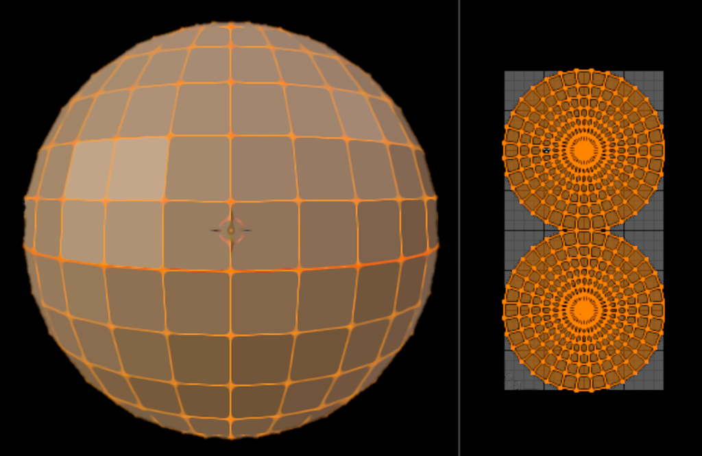
- UV Sphere: Uses rings of square faces to cut up the sphere, similar to the latitude and longitude lines used in cartography. While it approximates the surface of a sphere pretty well, the distribution of vertices is very uneven, especially at the poles and equator
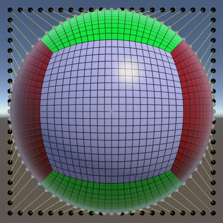
- Cube Sphere: Starts with a cube, whose faces are then tessellated, and the vertices are projected onto the surface of the sphere. The nice property of this mapping is that it enables an easy mapping of the sphere back onto the flat cube surfaces. But while it’s less unevenly distributed than UV-Spheres, the distribution is still far from uniform.
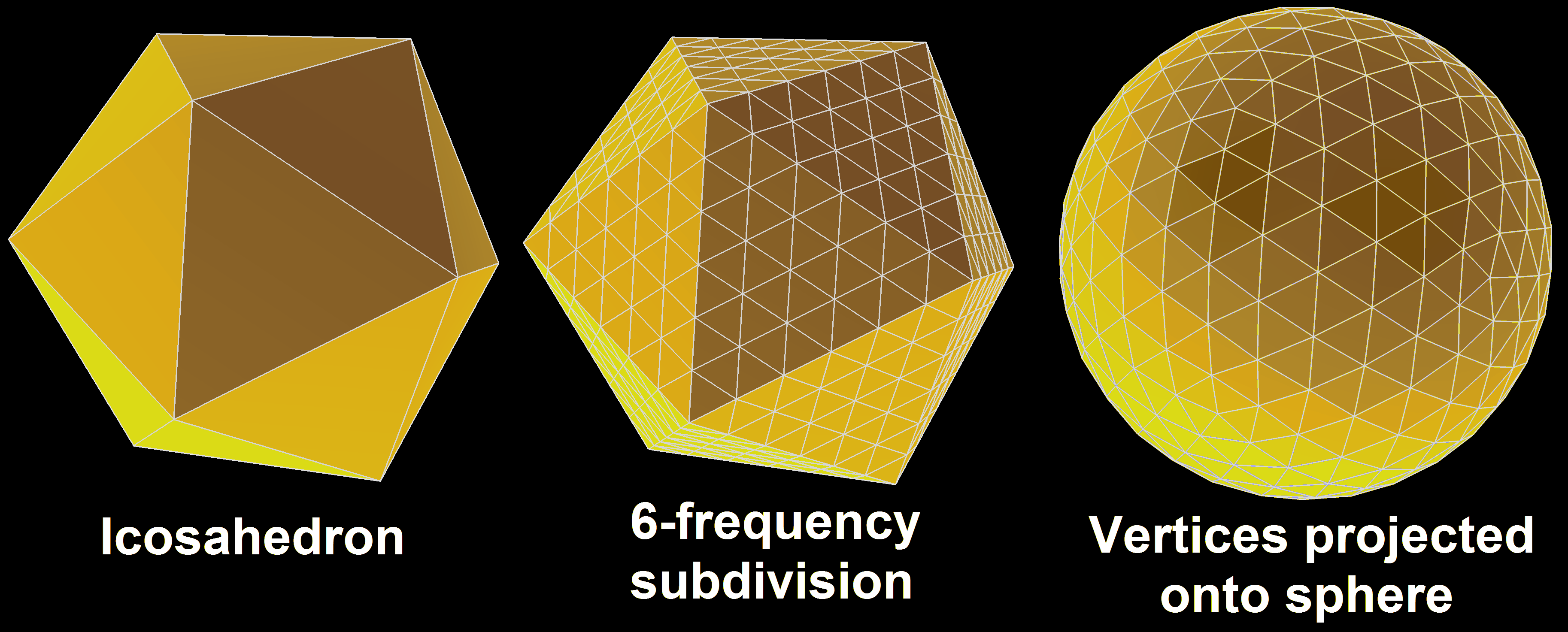
- Subdivided Icosahedron: This is probably the most common way to define a sphere mesh with evenly distributed vertices. The shape starts as an icosahedron with 12 vertices that loosely approximates the sphere. To get a better approximation, the next step is to subdivide its triangular faces into smaller triangles and then project each vertex onto the sphere’s surface. After a couple such subdivisions, this approximation gets relatively close to a real sphere, while the uniform distance between its vertices is conserved, which would make it a nice option for us. But a limitation of this approach is, that the number of vertices is defined by the number of subdivisions and increases quadratically (12, 42, 162, 642, 2562, …), which limits our options for the initial resolution more than I would prefer.
The subdivided Icosahedron would probably work for us, but I don’t particularly like the restrictive vertex count options forced upon us by the recursive subdivision. Hence, we’ll instead use Fibonacci Spheres, which have a similar nice uniform distribution, but are not limited to particular vertex counts.
I won’t go into too much detail about how they are computed, as others have already covered that far better than I probably could. But to put it simply, they utilize the golden spiral (aka the Fibonacci spiral) to uniformly distribute points on a surface. This is similar to the way some plants distribute their leaves or seeds, by placing each point radians[1] further along a spiral path from the center, where is the golden ratio. So for points in a 2D spherical coordinate system we would use something like:
Now all that is left to use this on the surface of our sphere is to extend it from 2D spherical coordinates to 3D Cartesian coordinates. This can be done by cutting the sphere into circles along the Y-axis, by deriving the Y coordinate directly from the current index . Based on the radius of the sphere, we can then derive the radius of the current circle and calculate X and Z from the angle given by the equation above. So for the unit sphere with radius 1 and points we get:
Combining all this, the code that generates our vertex positions looks like this:
// Define the data layer that contains the vertex positions in 3D Cartesian coordinates
constexpr auto position_info = Layer_info<Vec3, Layer_type::vertex>("position");

// Acquire all necessary resources from the world structure
auto mesh        = world.lock_mesh();
auto [positions] = world.lock_layer(position_info);
auto rand        = world.lock_random();

// Create N vertices
mesh->add_vertices(vertex_count);

// Pre-calculate the golden angle and the step-size for calculating y,
//   so we just need to multiply them with i in the loop
constexpr auto golden_angle = 2.f * std::numbers::pi_v<float> * (2.f - std::numbers::phi_v<float>);
const auto     step_size    = 2.f / (vertices - 1);

for(std::int32_t i = 0; i < vertices; i++) {
	// Calculate the x/y/z position of the current vertex on the unit sphere
	const auto y     = 1.f - step_size * i;
	const auto r     = std::sqrt(1 - y * y);
	const auto theta = golden_angle * i;
	const auto x     = std::cos(theta) * r;
	const auto z     = std::sin(theta) * r;

	// Set the vertex position (multiplying with the radius of our sphere)
	positions[Vertex(i)] = Vec3{x, y, z} * radius;
}
Until now, we only defined our vertices as a cloud of points without any connectivity. So, the next step is to compute the Delaunay triangulation of these points. There are again a couple of ways to achieve this, but the easiest is to utilize the fact that the Delaunay triangulation of points on the surface of a sphere is identical to the convex hull of said points. Thus, all that’s left to do is import a library that computes the convex hull. The library already gives us a list of faces, that we just need to pass onto the add_face() function of Mesh[2]:
quickhull::QuickHull<float> qh;
auto  hull    = qh.getConvexHull(&positions.begin()->x, positions.size(), false, true);
auto& indices = hull.getIndexBuffer();

for(std::size_t i = 0; i < indices.size(); i += 3) {
	mesh->add_face(indices[i], indices[i+1], indices[i+2]);
}
As can be seen in the images below, the vertices are distributed evenly on the surface … perhaps too evenly. In some cases we might want a more natural and less uniform look. This can be achieved easily by adding a small random offset (0 <= offset < 1.0) to the loop variable i before it’s used in the calculations:
const auto offset = perturbation > 0 ? rand->uniform(0.f, perturbation) : 0.f;
auto       ii    = std::min(i + offset, vertices - 1.f);
// then use ii instead of i in the body of the loop
Implementing add_face
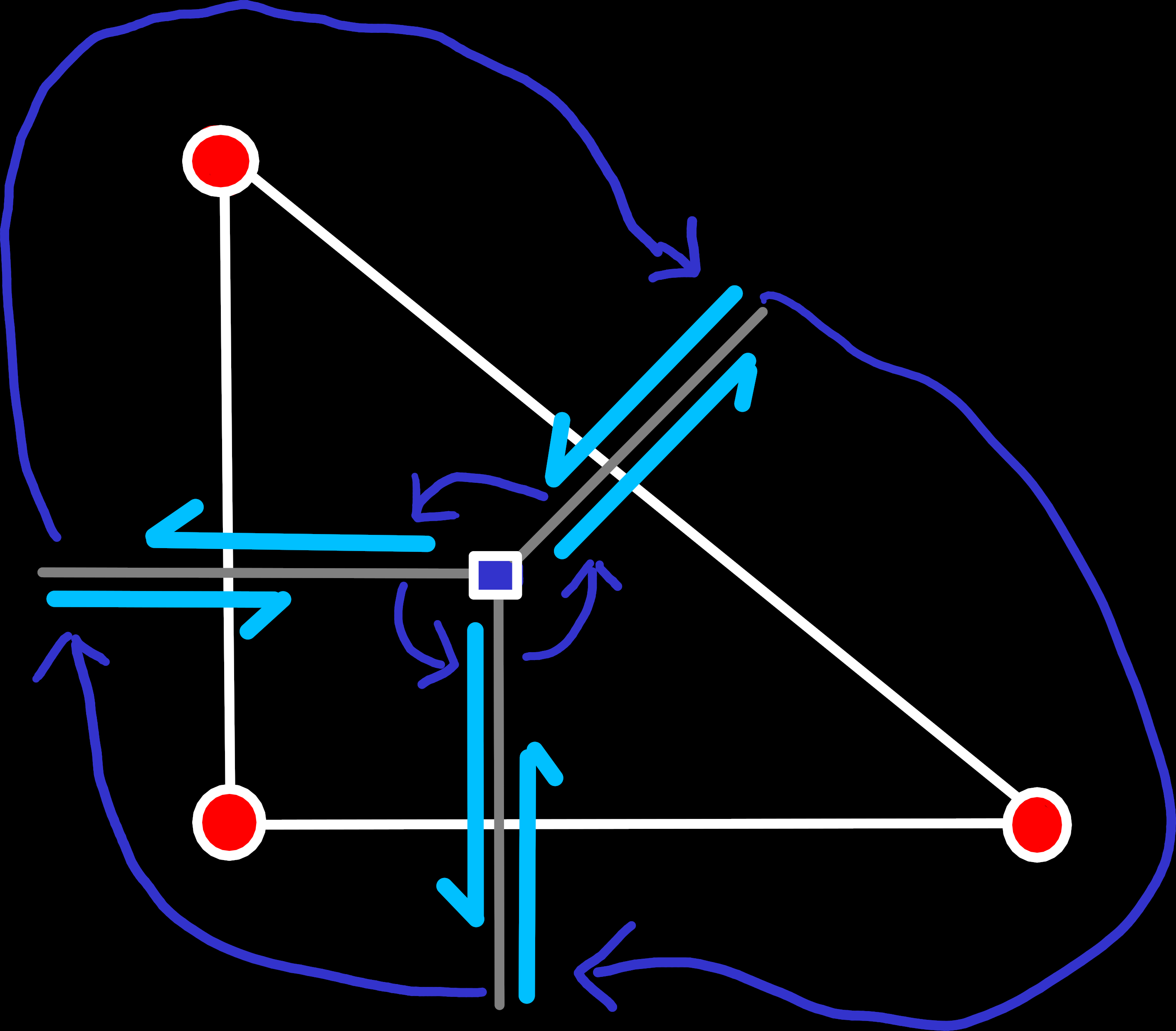
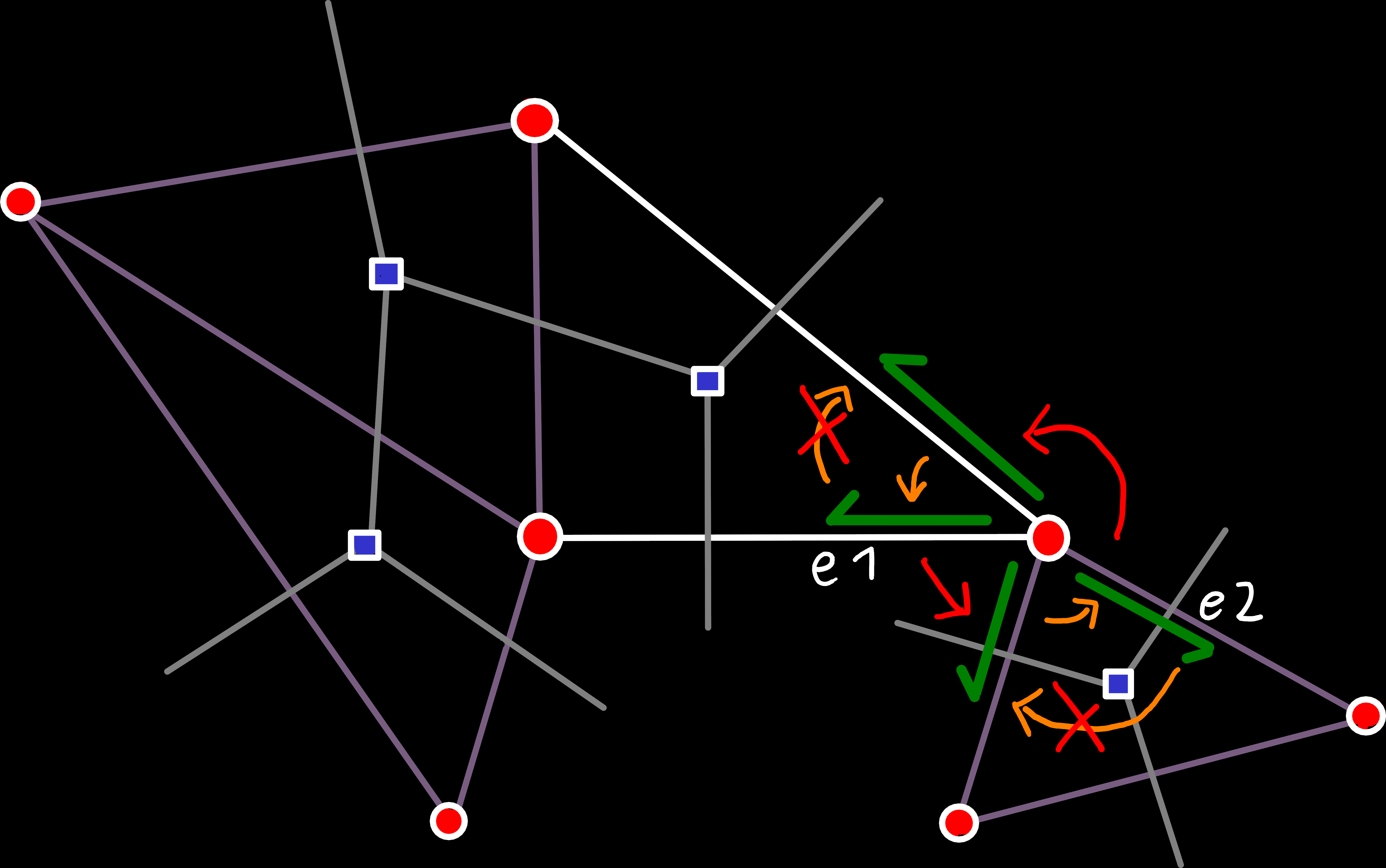
As said above, implementing this operation is not as straightforward as one might hope. The main problem is that triangles could be added in (nearly) any order, and we need to update the connectivity information correctly for all possible cases. Which boils down to updating the origin_next(e) references for all modified primal and dual edges, to preserve valid edge-rings, as visualized below.
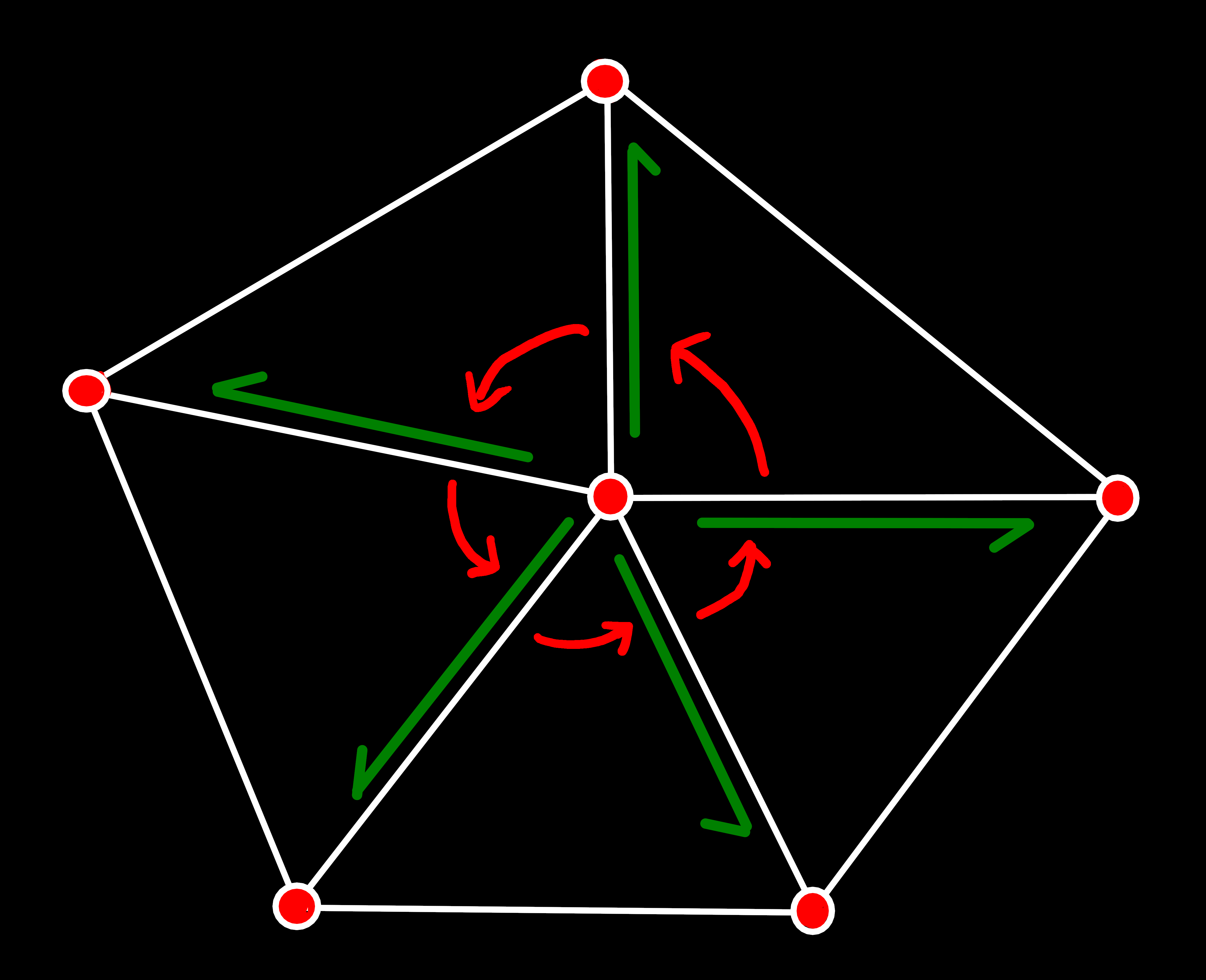
origin_next(e) for primal edges must always form an edge-ring that contains all primal edges with the same origin vertex, in counterclockwise order.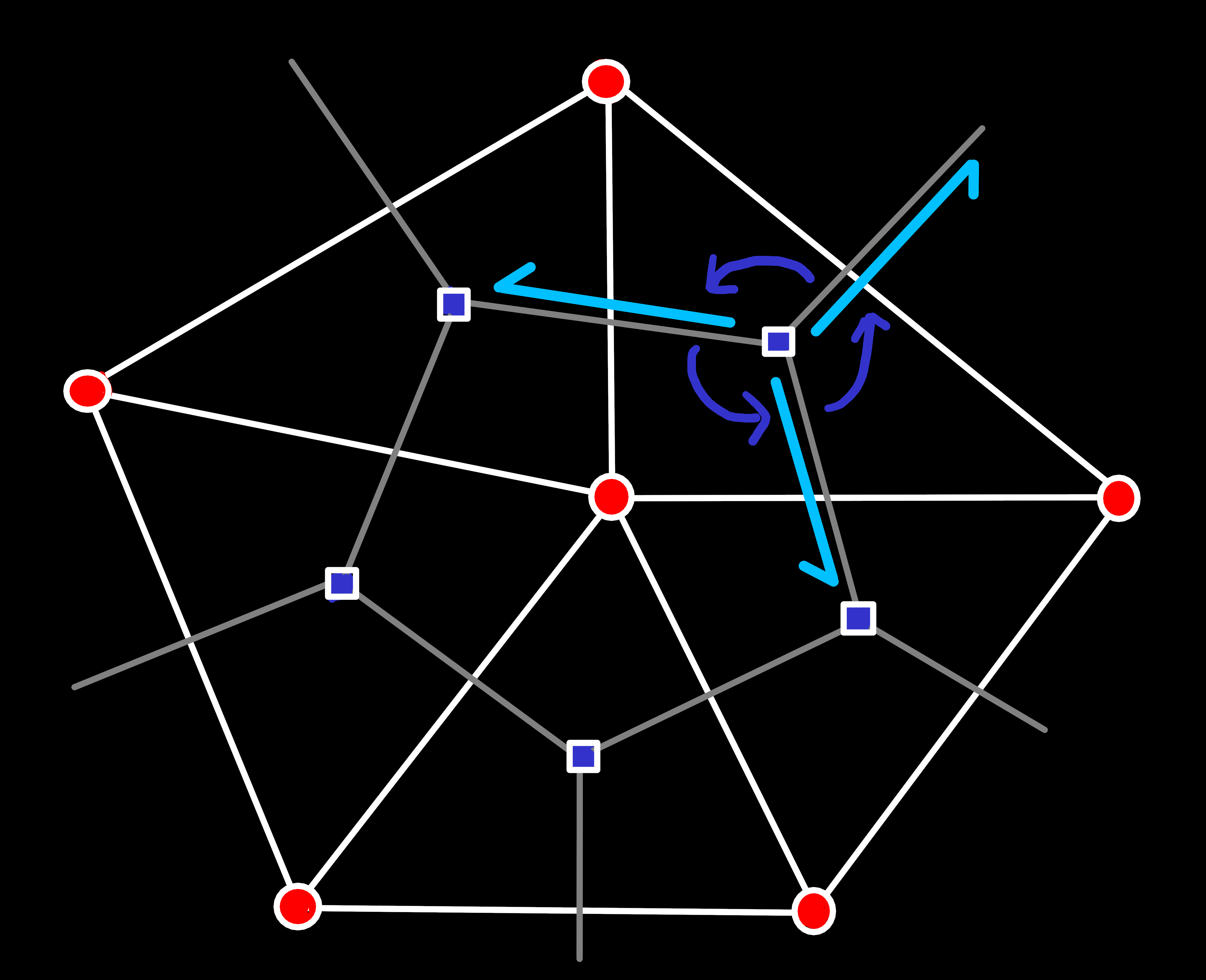
origin_next(e) for dual edges must form an edge-ring counterclockwise around a face.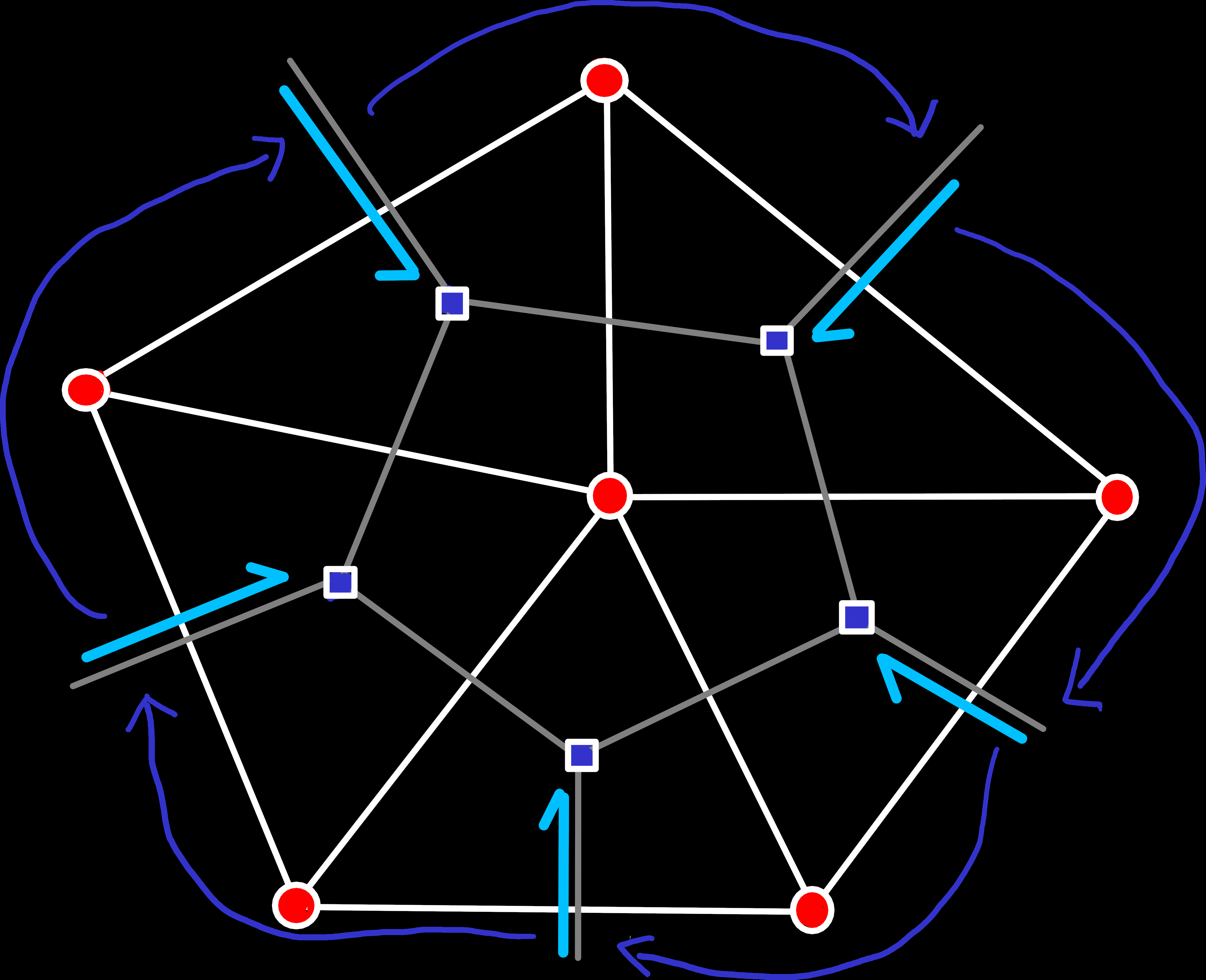
rot(e) of every boundary edge. While the order of the edges looks clockwise here, it's technically still counterclockwise, when seen from the perspective of the imaginary boundary face.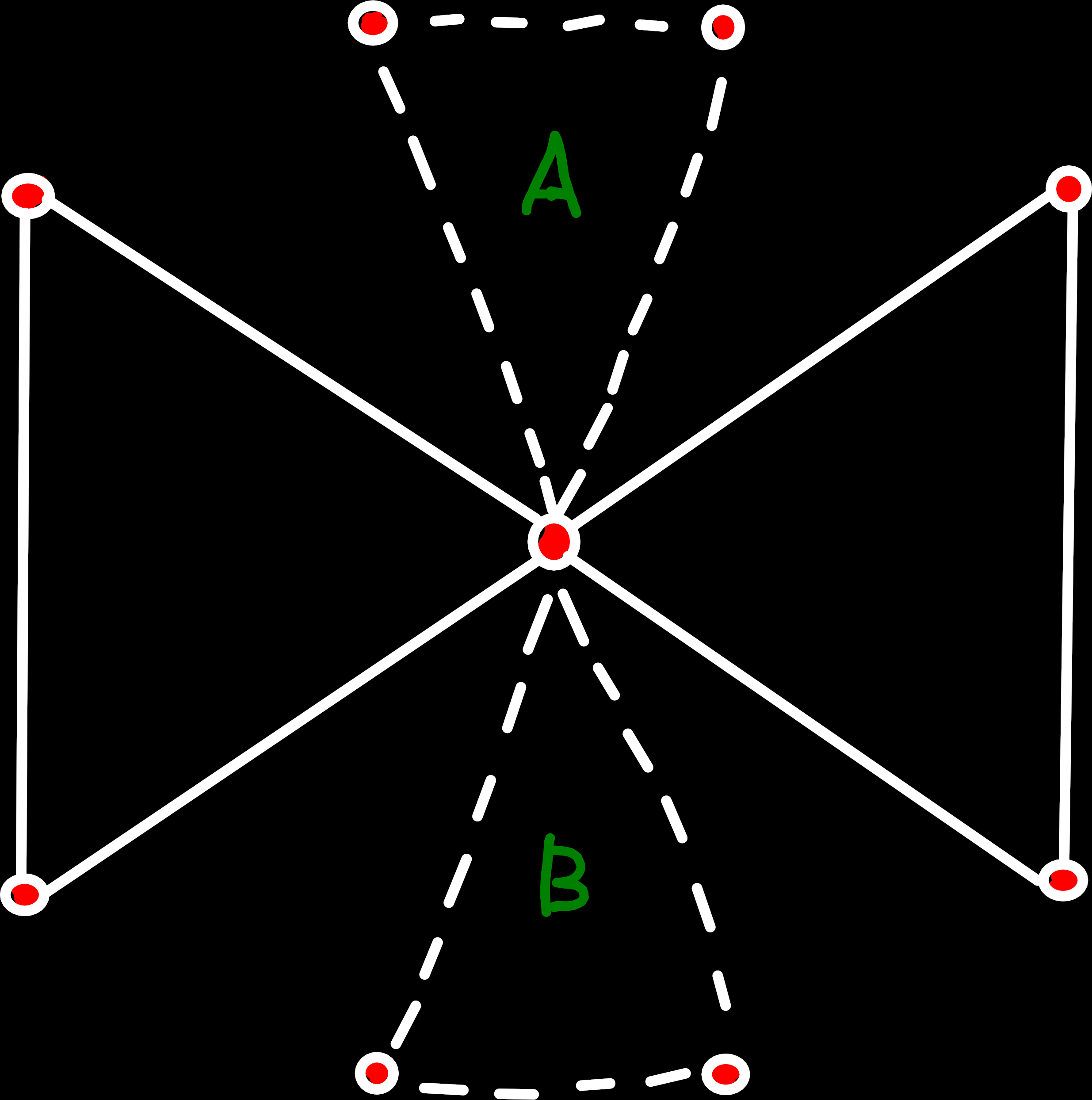
Because our mesh implementation doesn’t know about the position of vertices, we need to enforce one additional restriction on valid topologies: If multiple unconnected faces share a vertex, a new face can only be added to that vertex, if it also shares at least one edge with one of the existing faces. The problem we solve with this restriction is, that we have to know the order of the faces around a vertex, to be able to insert the edges at the correct positions in their new edge-rings. This ambiguity could[3] also be resolved by comparing the positions of the connected vertices. But this small restriction enables us to entirely ignore the vertex positions when working on the mesh and look at the topology only in terms of which vertices/faces are connected, without knowing how they will be laid out in space.
When we take all these restrictions into account and simplify the problem a bit, we only have to handle 8 different cases in total to add a new face to the mesh. One for each of the three quad-edges of the new face, that could either be missing or already exist. Luckily, most of these are rotationally symmetrical, and we only need to look at 4 distinct cases, that we can identify by counting the number of preexisting edges.
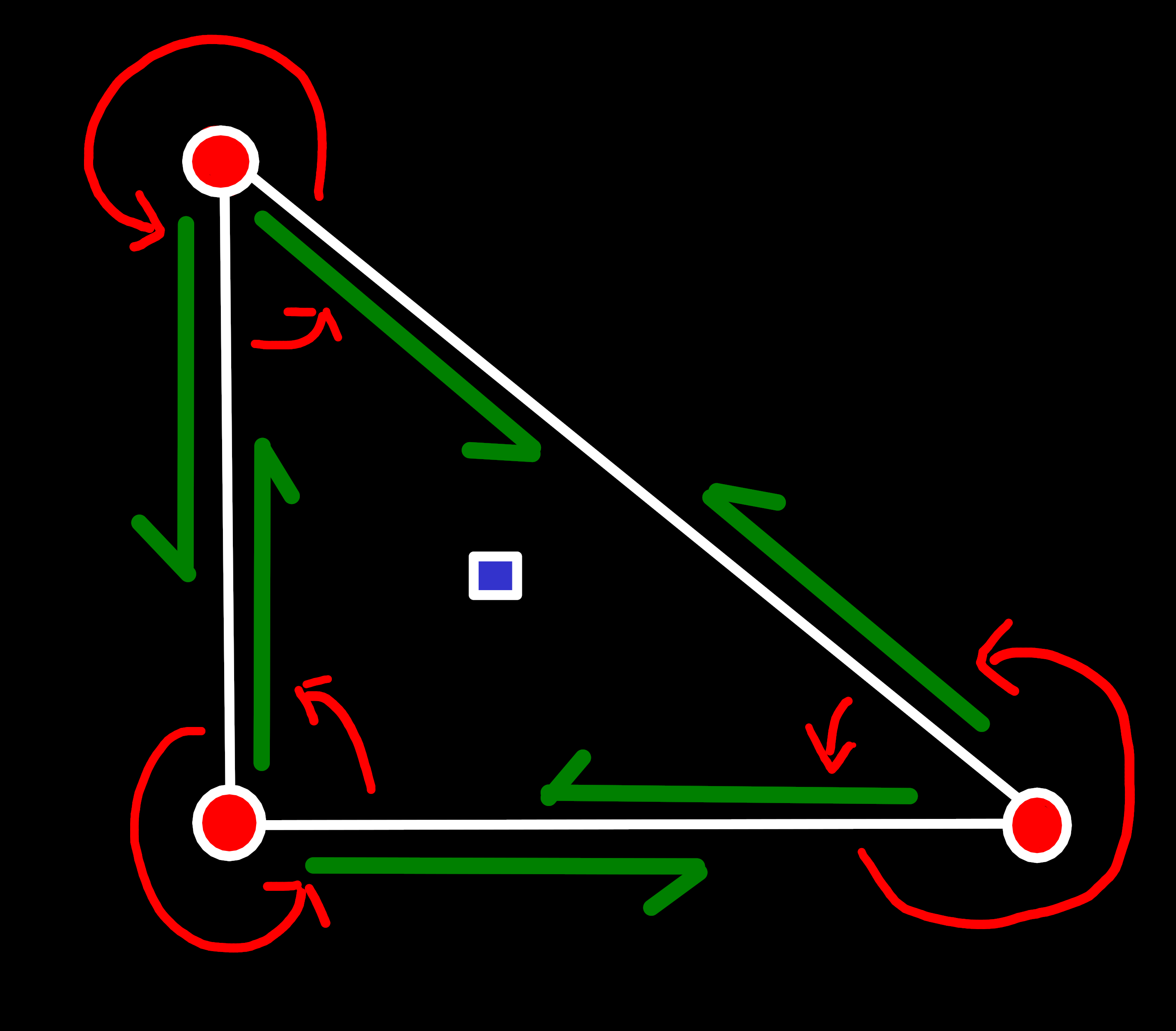
Case 0: No Preexisting Edges
The simplest case — and also the first one we need when we construct a new mesh — is the situation where we don’t have any faces or edges. All we need to do in this case is create one face and three quad-edges and connect them as shown below[4]:
Case 1: One Preexisting Edge (two new Edges)
The next case is a bit more complex: One of our edges already exists. What that means is that we add our face onto another face, with which we share a single edge.
The complexity here comes from the fact that we need to insert our new edges into existing edge-rings. To be exact, the complex part is finding the correct edge-ring and insert position, i.e. the edge that should be directly in front of us in the ring. In contrast, the insertion itself is relatively easy[5]:
void insert_after(Edge predecessor, Edge new_edge) {
	// Find the edge that currently comes after the predecessor,
	auto& predecessor_next = primal_edge_next_[predecessor.index()];

	// ... set that as our next edge and
	primal_edge_next_[new_edge.index()] = predecessor_next;

	// ... change the predecessor, so that it points to us
	predecessor_next = new_edge;
}
A relatively common case is that we know our successor but not our predecessor. In this case, we can just use origin_prev(e) to get its predecessor and insert ourselves between them. Though, one thing we need to keep in mind, is that the traversal operations won’t work as expected if we already modified part of the topology. So, the usual procedure is that we calculate and remember all information about the current topology that we will need and only modify it afterwards, whereby we achieve a consistent view of the topology.
void insert_before(Edge successor, Edge new_edge) {
	insert_after(successor.origin_prev(*this), new_edge);
}

insert_before() with e1,e2 and e3,e4.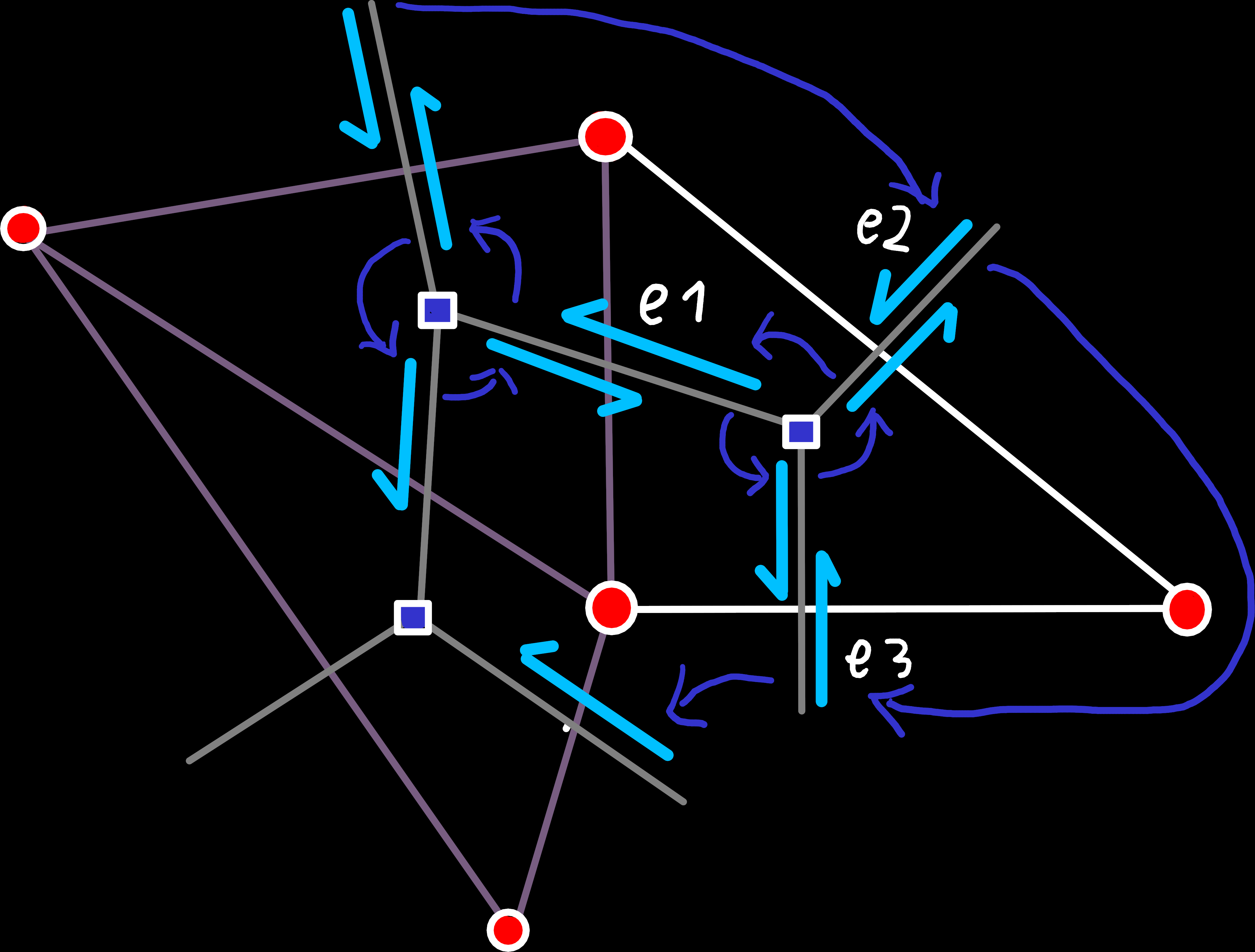
e1 was part of the boundary edge-ring. After the insertion that is no longer the case and e2 and e3 should be part of this edge-ring instead. So, we have to retrieve the predecessor of e1, let it point to e2, which points to e3, which finally points to the original successor of e1.Case 2: Two Preexisting Edges (one new Edge)
This case is quite similar to the previous one, but slightly simpler because we only have one newly created quad-edge that we need to connect. Thereby, the primal edge ring around one of the vertices is already correct, and we only need to update the other two to include the new edge. Wiring up the dual edges is the only part with a bit of complexity, but that case is also quite similar to case 1.
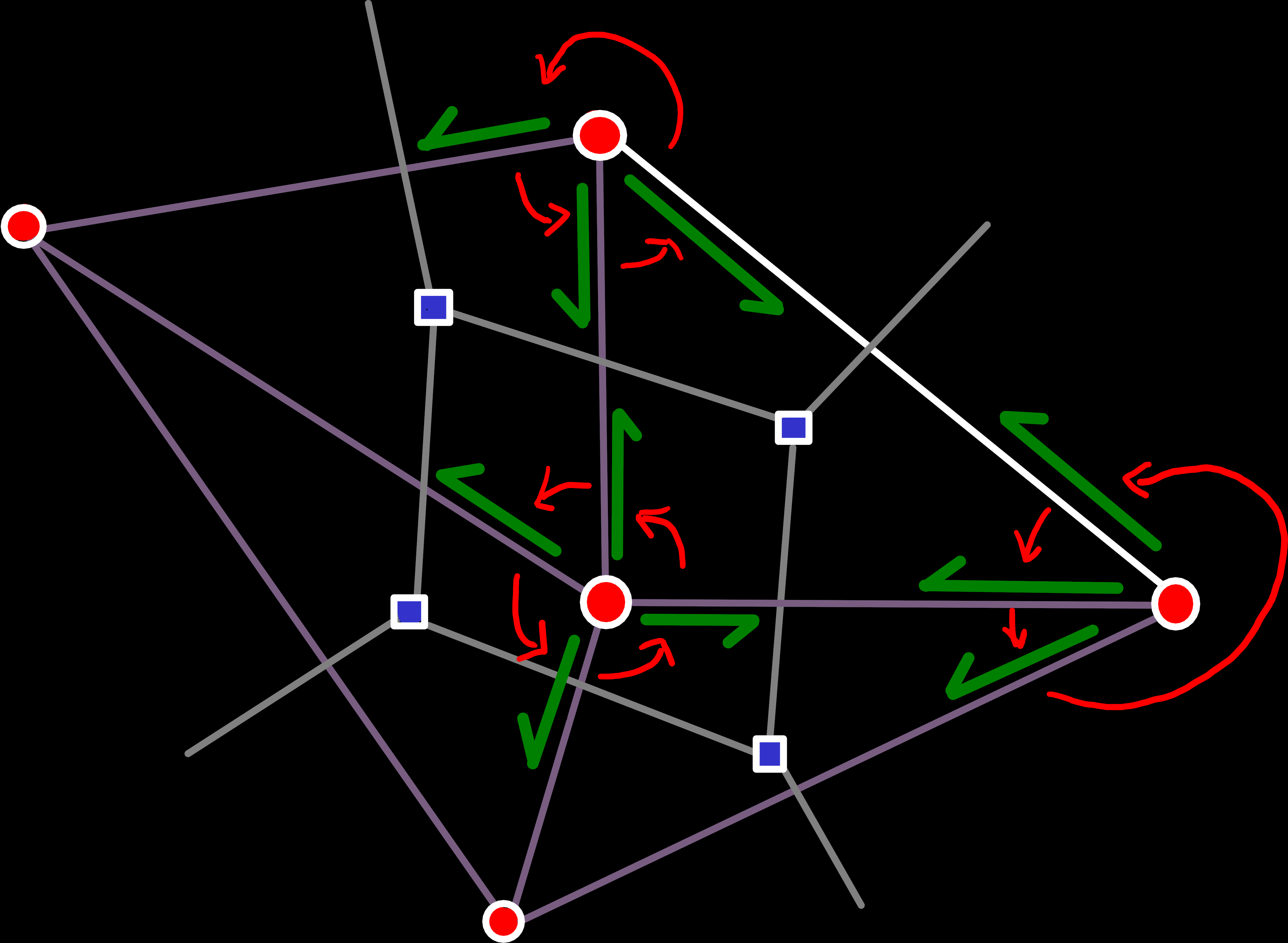
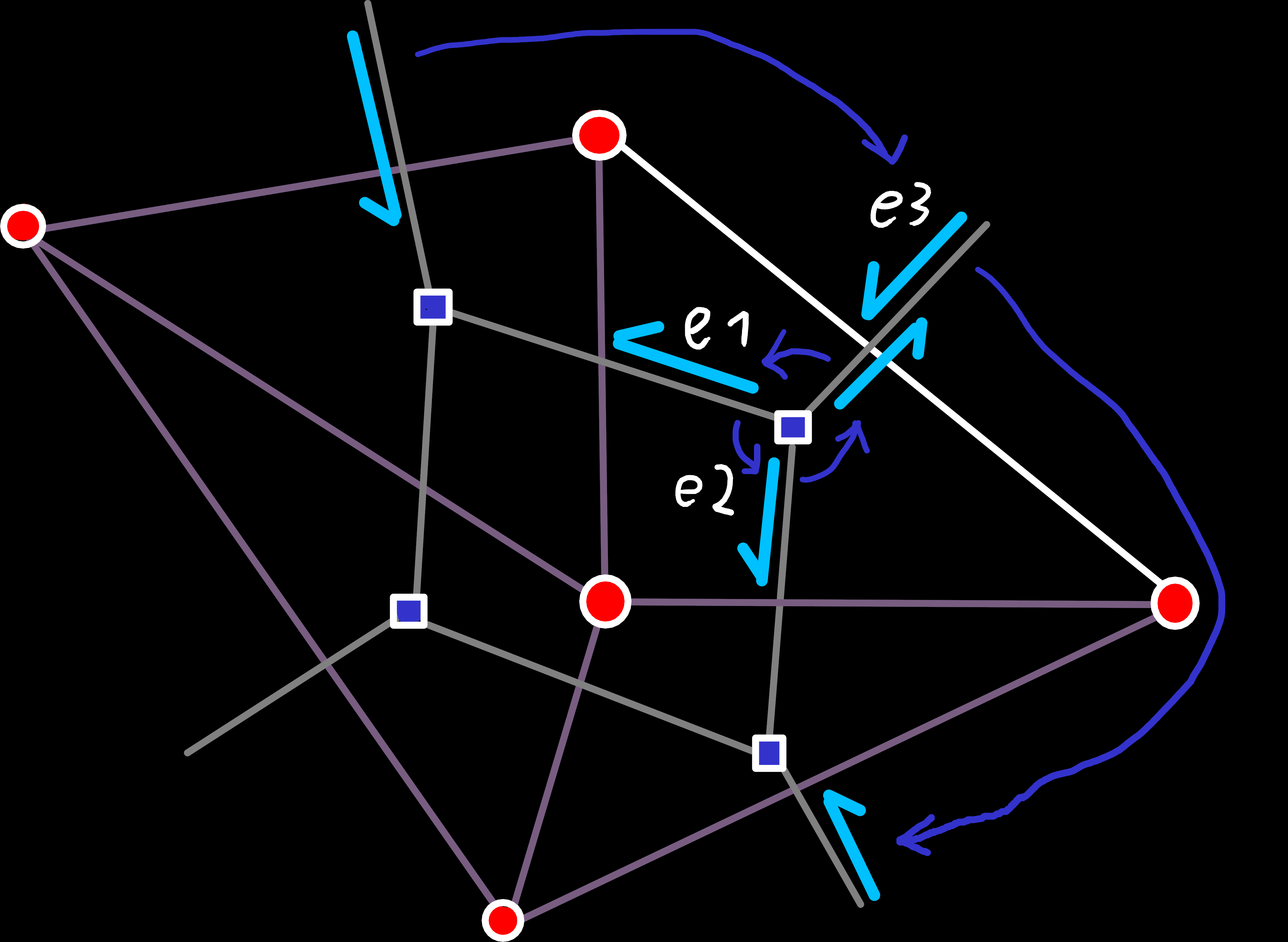
e1 and e2) and replace them with a single new edge (e3).Case 3: Three Preexisting Edges
The opposite of Case 1 is also simple enough: All three vertices of our face are already connected by edges, and we currently have a hole where we want to create the face. Because all connections are already established in this case, we don’t have to connect any edge, but just create a new face and set the origin of the dual edges leaving the face accordingly[6].
The Edge-Case[7]
We owe the simplicity of the previous cases primarily to one assumption: If a vertex is already part of a face, we share an edge with at least one of its faces.
But that assumption doesn’t hold in all cases. While our restriction from the beginning does forbid all cases where a vertex is shared by more than two unconnected faces, it leaves one case open that we still need to handle: A vertex that is shared by exactly two faces. We could’ve excluded that case too, of course. But in contrast to the others, this one is actually decidable based only on the topology. And by not allowing it we would unduly restrict the construction of meshes because without this case all new faces after the first one would have to share an edge with an existing face.
The reason that we’ve ignored this cases until now is that we can actually separate these concerns by splitting our function in two steps:
- Add the face like above, ignoring this special case
- Iterate over each affected vertex and fix the errors introduced by ignoring it
The specific errors that are introduced by this are unconnected edge-rings[8], which would cause massive problems during traversal because we would only see one of them when we iterate with origin_next(e). Luckily, we can solve this problem relatively easily by merging the two edge-rings:
void merge_edge_ring(Edge last_edge_of_a, Edge last_edge_of_b) {
	auto& a_next = primal_edge_next_[last_edge_of_a.index()];
	auto& b_next = primal_edge_next_[last_edge_of_b.index()];

	std::swap(a_next, b_next);
	// Now last_edge_of_a points to the first edge in b
	//  and last_edge_of_b points to the first edge in a
}
e1) and old edge-ring (e2). To do that here, we can just iterate over all edges of the respective ring, looking for the first edge that has no left face.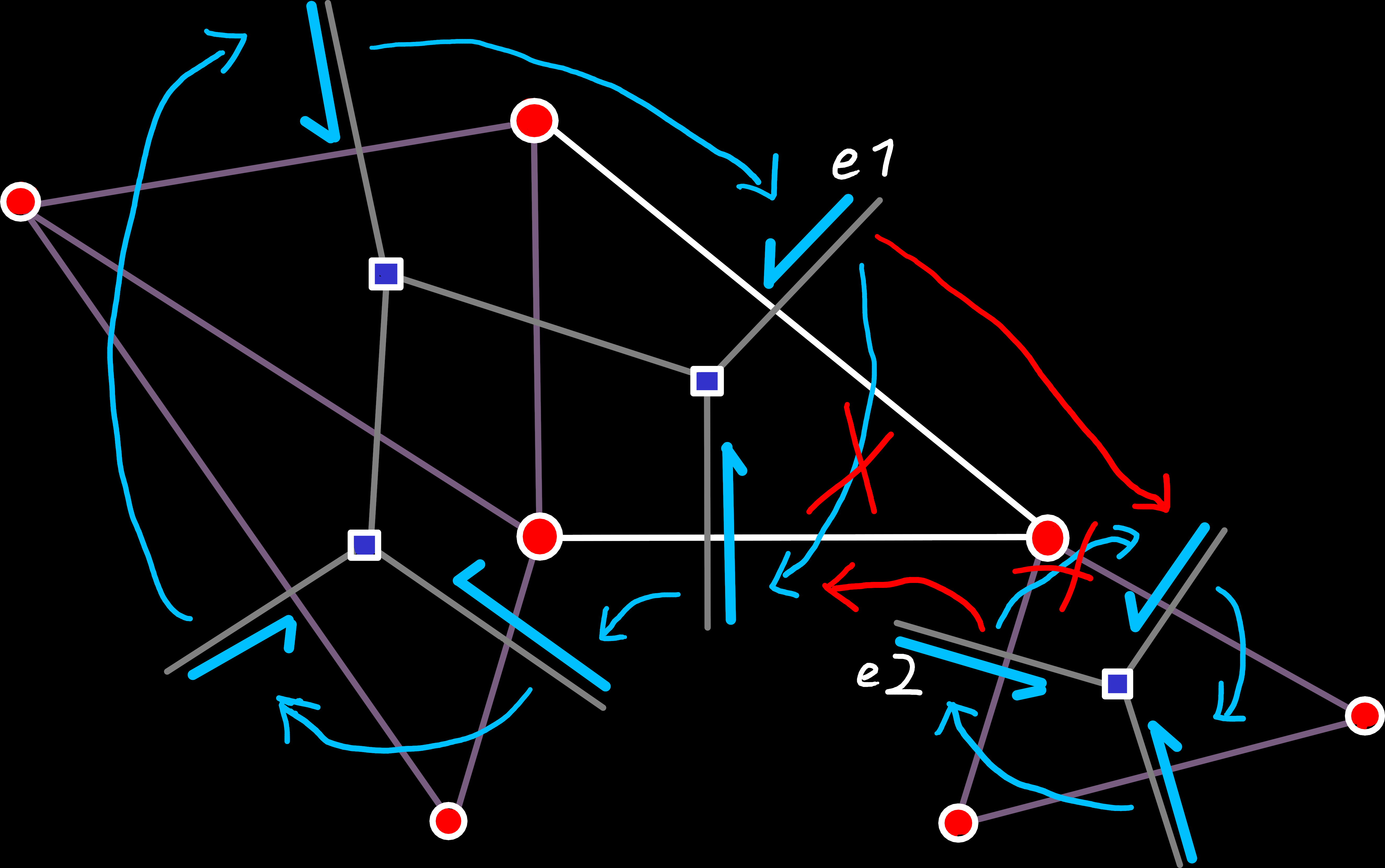
Conclusion
Now that we have our first world mesh, we can nearly start with the generation algorithms, like simulating plate tectonics. We’re just missing one final puzzle piece, we’ll look at next, that is the modification of our mesh during the simulation.